Frequentist and hybrid calibration of one-stage ROPE-based designs for single-arm phase II trials

Riko Kelter
Institute of Medical Statistics and Computational Biology
Faculty of Medicine
University of Cologne
Cologne, Germany

23 June 2026

Introduction

This vignette introduces the calibration of one-stage ROPE-based designs for single-arm phase II trials with binary endpoints, implemented in the function design_singlearm_onestage_rope(). In these trial types, the goal is to establish equivalence between a standard of care with success probability $p_0$ and a novel drug or treatment. For each patient, a failure or success is recorded in the single treatment arm, so the primary endpoint is binary. This offers flexibility and a wide range of applications.

The design is then based on a region of practical equivalence (ROPE) around the benchmark response probability $p_0$. The ROPE is defined as

$$\mathcal{R}_p = [p_0 - \delta,\; p_0 + \delta]\cap(0,1),$$

where $\delta > 0$ denotes the half-width of the ROPE. Equivalence is accepted when the posterior probability that $p$ lies inside the ROPE exceeds a chosen threshold,

$$\Pr(p \in \mathcal{R}_p \mid Y=y) \ge \gamma_{\mathrm{eq}}.$$

As for the Bayes-factor-based one-stage design, bfbin2arm provides four calibration modes for ROPE designs:

• Bayesian: Calibrate Bayesian predictive power and predictive type-I error.
• Frequentist: Calibrate frequentist power at a fixed point alternative and frequentist type-I error.
• Hybrid: Calibrate Bayesian predictive power and frequentist type-I error.
• Full: Calibrate all four operating characteristics simultaneously.

In addition, the ROPE design has three important tuning parameters that influence the frequentist operating characteristics:

• the posterior probability threshold $\gamma_{\mathrm{eq}}$,
• the ROPE half-width $\delta$,
• the point alternative $dp$ at which frequentist power is evaluated.

This vignette explains the calibration modes and illustrates the impact of these parameters in a worked example.

Design setup

We consider a single-arm phase II trial with a binary response. We formally test the hypotheses

$$H_0:p\in \mathcal{R}_p \text{ versus } H_1:p\notin \mathcal{R}_p$$

The null hypothesis $H_0$ implies that the novel drug or treatment is equivalent from a clinical perspective to the standard of care. The alternative hypothesis $H_1$ implies that it is not. In the latter case, the novel drug or treatment could either be substantially more effective or substantially less effective. In a phase II trial which aims to demonstrate equivalence between the standard of care and a novel drug or treatment, both of these results are undesirable.

The benchmark response probability is $p_0 = 0.30$, and the ROPE half-width is chosen as $\delta = 0.12$, so that

$$\mathcal{R}_p = [0.18, 0.42].$$

The analysis prior for the response probability is a $\mathrm{Beta}(1,1)$ distribution and is used to compute posterior ROPE probabilities at interim or final analysis. For calibration of predictive operating characteristics we use separate design priors under equivalence ($H_1$) and non-equivalence ($H_0$),

• under non-equivalence: $\mathrm{Beta}(60, 40)$,
• under equivalence: $\mathrm{Beta}(36, 84)$.

p0    <- 0.30
delta <- 0.12

a  <- 1;  b  <- 1    # analysis prior
da0 <- 60; db0 <- 40 # design prior under H0
da1 <- 36; db1 <- 84 # design prior under H1

The ROPE probability threshold $\gamma_{\mathrm{eq}}$ will be treated as a tuning parameter. In the examples below we will use $\gamma_{\mathrm{eq}} = 0.925$, which yields a design with Bayesian predictive power close to 0.8 and a frequentist type-I error near 0.1 under our specification.

Operating characteristics

For a fixed sample size $n$, the ROPE decision rule induces an equivalence acceptance region

$$\mathcal{A}_{\mathrm{eq}}(n) = \bigl\{ y \in \{0,\dots,n\} : \Pr(p \in \mathcal{R}_p \mid Y=y) \ge \gamma_{\mathrm{eq}} \bigr\}.$$

If the region is contiguous, we can write

$\mathcal{A}_{\mathrm{eq}}(n) = \{y_{\min}^{\mathrm{eq}}(n),\dots,y_{\max}^{\mathrm{eq}}(n)\}$.

Predictive (Bayesian) operating characteristics are computed under the design priors:

• predictive power under equivalence:

$$\mathrm{power}(n) = \Pr(\text{equivalence accepted} \mid H_1) = \sum_{y \in \mathcal{A}_{\mathrm{eq}}(n)} \Pr(Y=y \mid H_1),$$

• predictive type-I error under non-equivalence:

$$\mathrm{type1}(n) = \Pr(\text{equivalence accepted} \mid H_0) = \sum_{y \in \mathcal{A}_{\mathrm{eq}}(n)} \Pr(Y=y \mid H_0).$$

Frequentist operating characteristics are computed under fixed response probabilities:

• frequentist power at a point alternative $p \in \mathcal{R}_p$:

$$\mathrm{freq\_power}(n; p) = \Pr_{p}(\text{equivalence accepted}) = \sum_{y \in \mathcal{A}_{\mathrm{eq}}(n)} \binom{n}{y} p^y (1-p)^{n-y},$$

• frequentist type-I error at a point $p$:

$$\mathrm{freq\_type1}(n; p) = \Pr_p(\text{equivalence accepted}).$$

In this vignette, frequentist type-I error is defined as the worst case at the ROPE boundaries,

$$\mathrm{freq\_type1}^{\max}(n) = \max\{ \mathrm{freq\_type1}(n; p_0-\delta),\; \mathrm{freq\_type1}(n; p_0+\delta)\}.$$

The calibration modes select the sample size $n$ such that these operating characteristics meet specified targets.

Calibration modes

The function design_singlearm_onestage_rope() supports four calibration modes, specified via the argument calibration.

Bayesian calibration

In Bayesian mode, we calibrate the design using only the predictive operating characteristics under the design priors:

• predictive power under $H_1$ must be at least target_power,
• predictive type-I error under $H_0$ must be at most target_type1.

Frequentist power and frequentist type-I error are computed post hoc (if a point alternative dp is supplied), but they do not influence the selection of the sample size.

des_bayes <- design_singlearm_onestage_rope(
  n_min = 20,
  n_max = 300,
  p0 = p0,
  delta = delta,
  gamma_eq = 0.925,
  a = a, b = b,
  da0 = da0, db0 = db0,
  da1 = da1, db1 = db1,
  calibration = "Bayesian",
  target_power = 0.80,
  target_type1 = 0.10,
  sustain_n = 10
)

We can inspect the results as follows:

des_bayes

One-stage single-arm ROPE design
Calibration: Bayesian 
Search range n: 20 to 300 
Null probability p0: 0.3 
ROPE half-width delta: 0.12 
Probability threshold gamma_eq: 0.925 
Analysis prior: Beta(1, 1)
Design prior (H0): Beta(60, 40)
Design prior (H1): Beta(36, 84)
Target Bayesian power: 0.8 
Target Bayesian type-I error: 0.1 
Sustain n: 10 
Selected sample size n*: 173 
Bayesian power(n*): 0.8166 
Bayesian type-I(n*): 0.0001 
Equivalence region: [39, 63]

We can plot the results as follows:

plot(des_bayes)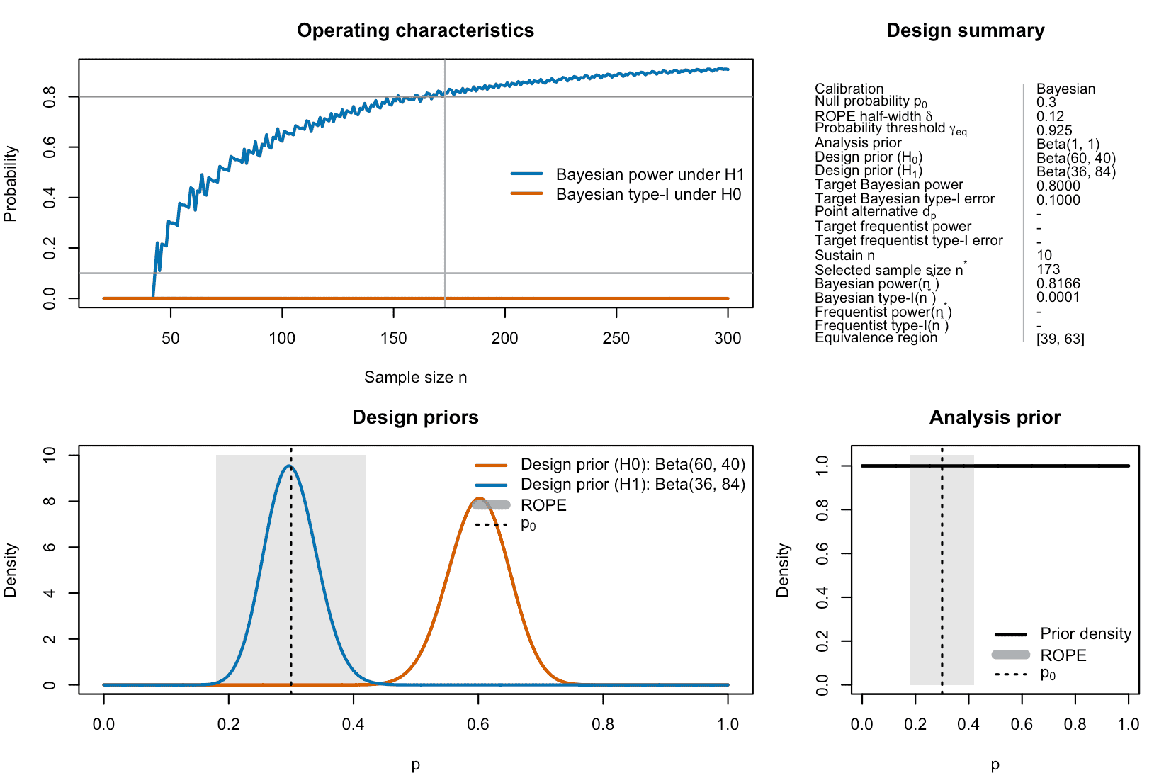

Figure 1: Bayesian calibration of a ROPE-based clinical phase II trial with binary endpoints.

The plot shows the selected sample size $n^\ast$, the predictive power and type-I error at $n^\ast$, and, if requested, frequentist quantities for comparison. As these are not requested, they are not shown in the upper right panel. The bottom left panel visualizes the design priors, the benchmark probability $p_0$ and the ROPE. The bottom right panel visualizes the analysis prior, the benchmark probability $p_0$ and the ROPE.

Frequentist calibration

In frequentist mode, we calibrate the design using frequentist power and frequentist type-I error only. This requires specification of a point alternative dp inside the ROPE:

• frequentist power at dp must be at least target_freq_power,
• frequentist type-I error (worst case at $p_0 \pm \delta$) must be at most target_freq_type1.

Bayesian predictive power and predictive type-I error are then reported post hoc.

des_freq <- design_singlearm_onestage_rope(
  n_min = 20,
  n_max = 300,
  p0 = p0,
  delta = delta,
  gamma_eq = 0.925,
  a = a, b = b,
  da0 = da0, db0 = db0,
  da1 = da1, db1 = db1,
  calibration = "frequentist",
  dp = 0.30,
  target_freq_power = 0.80,
  target_freq_type1 = 0.10,
  sustain_n = 10
)

des_freq

One-stage single-arm ROPE design
Calibration: frequentist 
Search range n: 20 to 300 
Null probability p0: 0.3 
ROPE half-width delta: 0.12 
Probability threshold gamma_eq: 0.925 
Analysis prior: Beta(1, 1)
Design prior (H0): Beta(60, 40)
Design prior (H1): Beta(36, 84)
Frequentist power point dp: 0.3 
Target frequentist power: 0.8 
Target frequentist type-I error: 0.1 
Sustain n: 10 
Selected sample size n*: 109 
Bayesian power(n*): 0.6755 
Bayesian type-I(n*): 0.0002 
Frequentist power(n*): 0.8227 
Frequentist type-I(n*): 0.0779 
  at p0 - delta: 0.0749 
  at p0 + delta: 0.0779 
Equivalence region: [26, 38] 

This mode is useful if regulatory or design requirements are expressed in terms of frequentist power and type-I error, while still employing a Bayesian ROPE decision rule in the analysis.

plot(des_freq)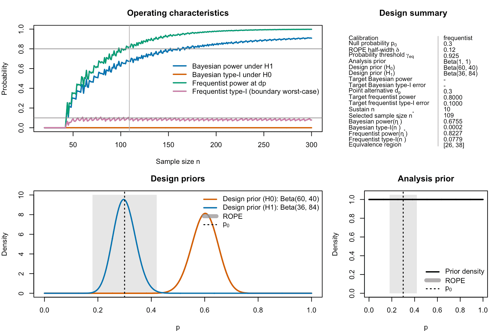

Figure 2: Frequentist calibration of a ROPE-based clinical phase II trial with binary endpoints. In contrast to Bayesian calibration, frequentist type-I-error rates are computed as worst-case scenarios at the ROPE-boundaries. Frequentist power is calculated under a specified point value for the success probability.

We can see that the selected sample size now shifts from $n^\ast$=173 when using Bayesian calibration to $n^\ast$=109 when using frequentist calibration.

Hybrid calibration

In hybrid mode, calibration combines a Bayesian power condition with a frequentist type-I constraint:

• predictive power under $H_1$ must be at least target_power,
• frequentist type-I error (worst case at $p_0 \pm \delta$) must be at most target_freq_type1.

Frequentist power and Bayesian predictive type-I error are computed and reported post hoc.

des_hybrid <- design_singlearm_onestage_rope(
  n_min = 20,
  n_max = 300,
  p0 = p0,
  delta = delta,
  gamma_eq = 0.925,
  a = a, b = b,
  da0 = da0, db0 = db0,
  da1 = da1, db1 = db1,
  calibration = "hybrid",
  dp = 0.30,
  target_power = 0.80,
  target_freq_type1 = 0.10,
  sustain_n = 10
)

des_hybrid

One-stage single-arm ROPE design
Calibration: hybrid 
Search range n: 20 to 300 
Null probability p0: 0.3 
ROPE half-width delta: 0.12 
Probability threshold gamma_eq: 0.925 
Analysis prior: Beta(1, 1)
Design prior (H0): Beta(60, 40)
Design prior (H1): Beta(36, 84)
Target Bayesian power: 0.8 
Frequentist power point dp: 0.3 
Target frequentist type-I error: 0.1 
Sustain n: 10 
Selected sample size n*: 173 
Bayesian power(n*): 0.8166 
Bayesian type-I(n*): 0.0001 
Frequentist power(n*): 0.9597 
Frequentist type-I(n*): 0.0784 
  at p0 - delta: 0.0755 
  at p0 + delta: 0.0784 
Equivalence region: [39, 63] 

plot(des_hybrid)

Figure 3: Hybrid calibration of a ROPE-based clinical phase II trial with binary endpoints. In hybrid calibration mode, Bayesian power is calibrated together with frequentist type-I-error, which often is required from a regulatory agencies perspective.

Hybrid calibration may be attractive when one wants to retain the prior-based predictive power criterion while explicitly limiting the frequentist type-I error at the ROPE boundary. The resulting sample size now is identical to the one obtained in the Bayesian calibration. The above plot shows why: Bayesian power is the limiting factor in this case, as frequentist type-I-error is calibrated already for much smaller sample sizes. Adjusting the design priors to be more informative could thus further reduce the required sample size in hybrid calibration, as Bayesian power then accumulates faster.

Full Bayes–frequentist calibration

In full mode, all four operating characteristics are used in calibration:

• predictive power under $H_1$ ≥ target_power,
• predictive type-I error under $H_0$ ≤ target_type1,
• frequentist power at dp ≥ target_freq_power,
• frequentist type-I error (worst case at $p_0 \pm \delta$) ≤ target_freq_type1.

This is the ROPE analogue of the “full Bayes–frequentist” calibration described for the Bayes factor design in the single-arm one-stage BF vignette.

des_full <- design_singlearm_onestage_rope(
  n_min = 20,
  n_max = 300,
  p0 = p0,
  delta = delta,
  gamma_eq = 0.925,
  a = a, b = b,
  da0 = da0, db0 = db0,
  da1 = da1, db1 = db1,
  calibration = "full",
  dp = 0.30,
  target_power = 0.80,
  target_type1 = 0.10,
  target_freq_power = 0.80,
  target_freq_type1 = 0.10,
  sustain_n = 10
)

print(des_full)

plot(des_full)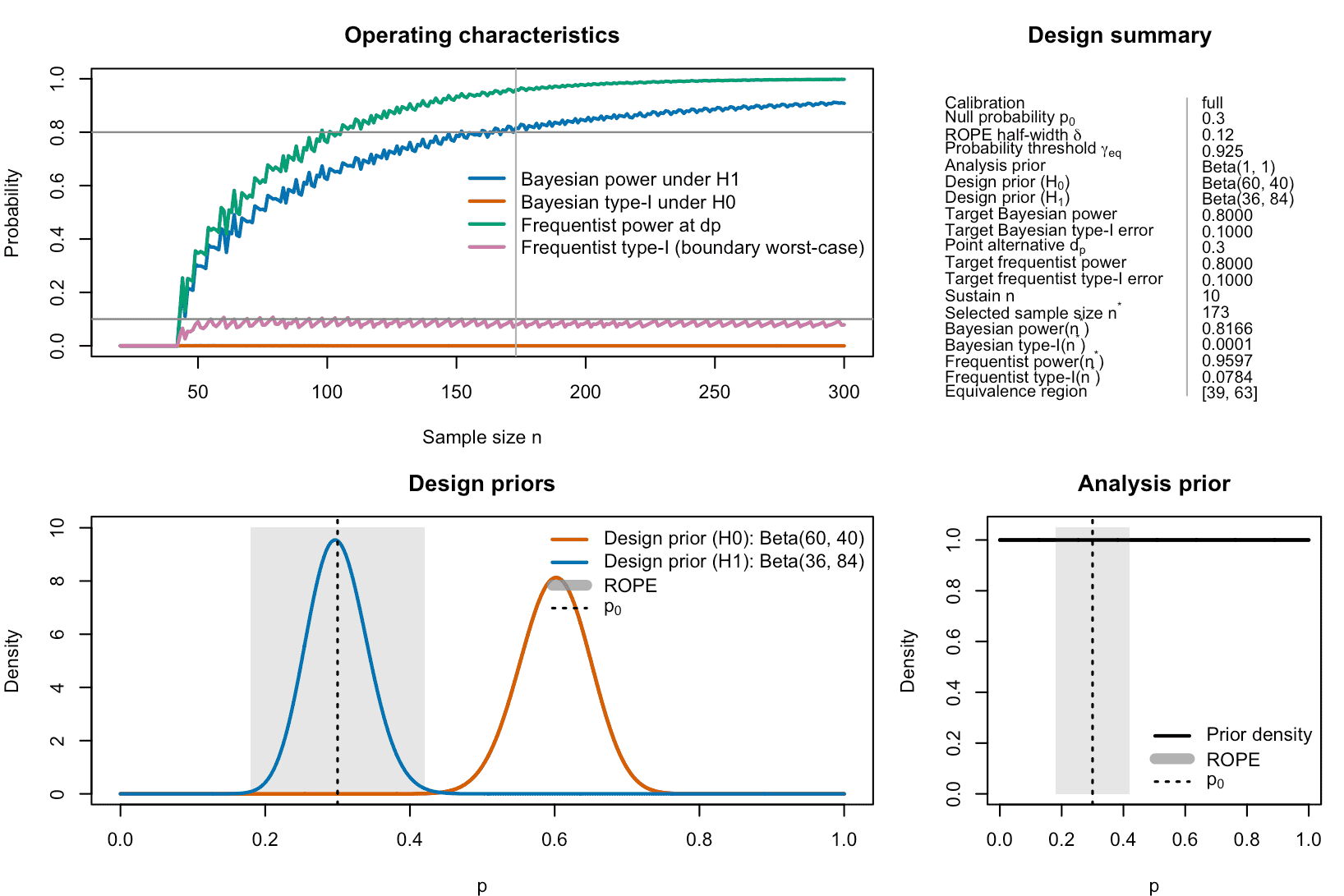

Figure 4: Full calibration of a ROPE-based clinical phase II trial with binary endpoints. In full calibration mode, Bayesian and frequentist power and type-I-error must be calibrated simultaneously, which is the strongest form of calibration.

For the chosen priors, ROPE width, and $\gamma_{\mathrm{eq}} = 0.925$, this yields a design with:

• $n^\ast = 173$,
• predictive power ≈ 0.82 under $H_1$,
• predictive type-I error ≈ 0.0001 under $H_0$,
• frequentist power ≈ 0.96 at $dp = 0.30$,
• frequentist type-I error ≈ 0.078 at the ROPE boundary.

The sustainable feasibility requirement (sustain_n = 10) ensures that the operating characteristics remain within target bounds for several larger sample sizes as well.

Tuning parameters for frequentist calibration

When using calibration modes that involve frequentist operating characteristics, three parameters play a central role:

1. the ROPE probability threshold $\gamma_{\mathrm{eq}}$,
2. the ROPE half-width $\delta$,
3. the point alternative $dp$.

The posterior probability threshold $\gamma_{\mathrm{eq}}$

The threshold $\gamma_{\mathrm{eq}}$ controls how demanding the ROPE decision rule is. It is the posterior probability which is required to be located inside the ROPE to establish equivalence. Larger values of $\gamma_{\mathrm{eq}}$ shrink the set of $y$ for which equivalence is accepted, which:

• decreases frequentist type-I error at the ROPE boundary,
• typically decreases predictive power and frequentist power as well.

In the current example, setting $\gamma_{\mathrm{eq}} = 0.8$ leads to a frequentist type-I error around 0.20–0.23 at the ROPE boundary, which is incompatible with a target of 0.10. Increasing the threshold to $\gamma_{\mathrm{eq}} = 0.925$ yields a boundary-based frequentist type-I error around 0.08, compatible with a 0.10 target, while still achieving predictive and frequentist power values above 0.8.

Users can treat $\gamma_{\mathrm{eq}}$ as a tuning parameter (similar to a Bayes factor threshold) and explore its impact on operating characteristics:

gamma_grid <- c(0.80, 0.85, 0.90, 0.925, 0.95)

res_gamma <- lapply(gamma_grid, function(gam) {
  design_singlearm_onestage_rope(
    n_min = 20, n_max = 300,
    p0 = p0, delta = delta, gamma_eq = gam,
    a = a, b = b,
    da0 = da0, db0 = db0,
    da1 = da1, db1 = db1,
    calibration = "frequentist",
    dp = 0.30,
    target_freq_power = 0.80,
    target_freq_type1 = 0.10,
    sustain_n = 10
  )
})

The ROPE half-width $\delta$

The ROPE half-width $\delta$ encodes what is considered “clinically equivalent” to $p_0$. A narrower ROPE:

• makes equivalence harder to achieve,
• tends to reduce frequentist type-I error at the boundary,
• but also reduces power to declare equivalence when the true $p$ is only moderately different from $p_0$.

Conversely, a wider ROPE relaxes the equivalence notion but may increase frequentist type-I error and require more careful calibration of $\gamma_{\mathrm{eq}}$.

Users can combine changes in $\delta$ and $\gamma_{\mathrm{eq}}$ to achieve desired trade-offs between clinical tolerance and statistical error control.

The Point alternative $dp$

The point alternative dp determines where frequentist power is evaluated. It should lie inside the ROPE, for example at the center (dp = p0) or at a clinically relevant equivalence point.

In frequentist or full calibration modes:

• dp must be specified,
• frequentist power at dp is calibrated to exceed target_freq_power.

For pure Bayesian or hybrid calibration, dp is optional. If supplied, the design function reports frequentist power at dp post hoc. Choosing dp near the center of the ROPE emphasizes performance when the true response probability lies well inside the equivalence region; choosing dp closer to a ROPE boundary focuses on performance near the edge of equivalence.

Summary

The ROPE-based one-stage design in bfbin2arm supports the same four calibration modes as the Bayes-factor-based design:

• purely Bayesian,
• purely frequentist,
• hybrid,
• full Bayes–frequentist.

For the frequentist and full calibration modes, the interplay of the ROPE threshold $\gamma_{\mathrm{eq}}$, the ROPE width $\delta$, and the point alternative dp determines whether both Bayesian and frequentist operating characteristics can reach their targets simultaneously. The current vignette illustrates how to specify these parameters and interpret the resulting operating characteristics for a typical single-arm phase II scenario.