Bayesian calibration of two-arm one-stage Bayes factor designs with binary endpoints

Riko Kelter
Institute of Medical Statistics and Computational Biology
Faculty of Medicine
University of Cologne
Cologne, Germany

23 June 2026

Introduction and Overview

In this vignette, we illustrate how to calibrate a two-arm one stage phase II design with binary endpoints from a Bayesian perspective. Details on the methodology can be found in (Kelter 2026). Our main assumption here is that the observed data in both groups are from two random variables $Y_1,Y_2$ which both follow a binomial distribution with parameters $n_1$ and $n_2$ and $p_1$ respectively $p_2$, $$Y_1\sim \mathrm{Bin}(n_1,p_1), \hspace{1cm} Y_2\sim \mathrm{Bin}(n_2,p_2)$$

Hypothesis tests

In its current form, the package implements four different hypothesis tests for such trials:

$$H_0:p_1=p_2 \hspace{1cm} \text{ versus } \hspace{1cm} H_1:p_1\neq p_2$$

Alternatively, a well-known parameterization of this test introduces a difference parameter $\eta=p_2-p_1$ and the grand mean $\zeta=\frac{1}{2}(p_1+p_2)$. Using this parameterization, we have

$$p_1=\zeta-\frac{\eta}{2}, \hspace{1cm} p_2=\zeta+\frac{\eta}{2}$$

and the hypotheses can be rewritten as:

$$H_0:\eta = 0 \hspace{1cm} \text{ versus } \hspace{1cm} H_1:\eta \neq 0$$

Next to this two-sided test, three directional tests are available in the package:

• $$H_0:\eta \leq 0 \hspace{1cm} \text{ versus } \hspace{1cm} H_1:\eta > 0$$
• $$H_0:\eta = 0 \hspace{1cm} \text{ versus } \hspace{1cm} H_1:\eta > 0$$
• $$H_0:\eta = 0 \hspace{1cm} \text{ versus } \hspace{1cm} H_1:\eta < 0$$

For each of the four tests, a separate Bayes factor exists and can be used. For the two-sided test, we denote the Bayes factor as $BF_{01}$, and for the three directional tests above we denote the Bayes factors as $BF_{+-}$, $BF_{+0}$ and $BF_{-0}$. Thus, the test of $H_0:\eta \leq 0$ versus $H_1:\eta >0$ can also be written as $H_-:p_2 \leq p_1$ versus $H_+:p_2 > p_1$.

Design and analysis priors

The $\mathrm{Beta}(a_0,b_0)$ distribution is a conjugate prior for the binomial likelihood, and when chosen as the prior, the posterior $P_{p \mid Y}$ is also Beta-distributed. A natural choice for the priors is the beta distribution. We assume independent Beta design priors $H_0$ as follows:

$$p_1 =p_2 = p\mid H_0 \sim \mathrm{Beta}(a_0^d,b_0^d)$$

Thus, under $H_0:\eta = 0$, both probabilities are identical, $p_1=p_2$, and take some value $p\in [0,1]$, which has a beta design prior. Likewise, we pick independent Beta design priors under $H_1:\eta \neq 0$:

$$p_1 \mid H_1 \sim \mathrm{Beta}(a_1^d,b_1^d), \hspace{1cm} p_2 \mid H_1 \sim \mathrm{Beta}(a_2^d,b_2^d)$$

For the analysis priors $P_{p_1}^a$, $P_{p_2}^a$ under $H_1$, we also choose independent Beta priors, with possibly different values $a_i^a$ and $b_i^a$ for $i=1,2$, where the superscript signals that the hyperparameters belong to our analysis instead of design prior:

$$p_1 \mid H_1 \sim \mathrm{Beta}(a_1^a,b_1^a), \hspace{1cm} p_2 \mid H_1 \sim \mathrm{Beta}(a_1^a,b_1^a)$$

Lastly, for the analysis prior $P_{p}^a$ under $H_0:\eta=0$, we choose a Dirac prior with all probability on $\eta=p_2-p_1=0$ conditionally on a uniform prior on $\zeta$, that is

$$p_1=p_2=p|H_0 \sim 1_{\{\eta=0\}}| \zeta \sim U(0,1)$$

for the analysis with the Bayes factor.

Using the package

First, we load the package after installation:

library(bfbin2arm)

Next, we illustrate the main calibration function for a two-arm one-stage trial by re-analyzing a phase II trial in the context of oncology. While no Bayesian approach was used in the original statistical analysis of the trial, the step-by-step walktrough below showcases how a structured approach to designing and calibrating a Bayesian two-arm one-stage phase II trial with the bfbin2arm package looks like. Importantly, the trial must have two trial arms (treatment and control) and binary endpoints. We assume further that one of the four tests detailed above is carried out using Bayes factors as the test criterion.

ICT-107 Phase II Trial Overview

The ICT-107 trial (Wen et al. 2019) was a randomized phase II study in newly diagnosed glioblastoma patients (n=124, 2:1 randomization). The primary binary endpoint is progression status at 6 months (PFS6), and the secondary binary endpoint immunologic status. Here, we focus on the secondary endpoint for illustration purposes.

Reported results (ITT population):

• ICT-107 (n=82): 49/82 responders= 59.7% response rate
• Control (n=42): 12/42 responders = 35.7% response rate

1. Bayes Factor Analysis

We start by calculating the Bayes factor(s) for the ICT-107 trial data:

## -------------------------------------------------------------
## 2. ICT-107 trial (immunologic response)
##    Placebo (control): 12 responders, 31 non-responders
##    ICT-107 (treatment): 49 responders, 32 non-responders  
## -------------------------------------------------------------

y1_ict <- 12      # control successes
n1_ict <- 12 + 31
y2_ict <- 49      # treatment successes
n2_ict <- 49 + 32

cat("\n=== ICT-107 Trial (n1 =", n1_ict, ", n2 =", n2_ict, ") ===\n")
#> 
#> === ICT-107 Trial (n1 = 43 , n2 = 81 ) ===

# BF01
BF01_ict = twoarmbinbf01(y1_ict, y2_ict, n1_ict, n2_ict, 
                         a_0_a = 1, b_0_a = 1, 
                         a_1_a = 1, b_1_a = 1, 
                         a_2_a = 1, b_2_a = 1)

# BF+1
BFp1_ict = BFplus1(y1_ict, y2_ict, n1_ict, n2_ict, 
                   a_1_a = 1, b_1_a = 1, 
                   a_2_a = 1, b_2_a = 1)

# BF-1
BFm1_ict = BFminus1(y1_ict, y2_ict, n1_ict, n2_ict, 
                    a_1_a = 1, b_1_a = 1, 
                    a_2_a = 1, b_2_a = 1)

# BF+0
cat("=== ICT-107 Trial === Bayes factor BF+0 results in ", BFplus0(BFp1_ict, BF01_ict))
#> === ICT-107 Trial === Bayes factor BF+0 results in  186.6192

# BF+-
cat("=== ICT-107 Trial === Bayes factor BF+- results in ", BFplusMinus(BFp1_ict, BFm1_ict))
#> === ICT-107 Trial === Bayes factor BF+- results in  3702.659

The most relevant Bayes factor here is $BF_{+-}$, because it is directional and leaves open the possibility of the placebo group having a larger response rate than the treatment group. Note that the hyperparameters of the beta analysis priors are specified in twoarmbinbf01 via a_0_a = 1, b_0_a = 1 et cetera.

2. Operating characteristics for actual sample sizes

Now, a key question is which operating characteristics can be expected based on the actual sample sizes used in the trial. The powertwoarmbinbf01 function can provide the answer:

ict_results <- powertwoarmbinbf01(
  n1 = n1_ict, n2 = n2_ict,
  k = 1/3, k_f = 3,
  test = "BF+-",  # H+: p2 > p1 vs H-: p2 <= p1
  a_0_d = 1, b_0_d = 1, a_0_a = 1, b_0_a = 1,
  a_1_d = 1, b_1_d = 1, a_2_d = 1, b_2_d = 1,
  a_1_a = 1, b_1_a = 1, a_2_a = 1, b_2_a = 1,
  output = "numeric",
  compute_freq_t1e = TRUE,
)
print(ict_results)

Power             Type1_Error 
              0.8788106               0.0214111 
                  CE_H0 Frequentist_Type1_Error 
              0.8788106               0.2871811 
attr(,"hypothesis")
[1] "H[+]:~p[2] > p[1] ~~ vs ~~ H[-]:~p[2] <= p[1]"
attr(,"compute_freq_t1e")
[1] TRUE

We see that based on the actual sample sizes and a moderate evidence threshold $k=1/3$, the Bayesian power is sufficiently large with $87.8\%$. Still, the frequentist type-I-error rate is way too high with $28.7\%$, so we increase the evidence threshold to $k=1/10$ (strong evidence) and use the ntwoarmbinbf01 function to calibrate the design based on our requirements next.

3. Power and sample size planning

The core working function to design a Bayesian two-arm one-stage trial with the package is the design_twoarm_onestage_bf() function. It searches over a grid of total sample sizes and returns a design object that contains

• the selected sample sizes in each arm (n1, n2) and their sum (n_total)
• Bayesian and frequentist operating characteristics at the chosen design
• the full search grid with pointwise and sustained feasibility indicators
• the calibration targets and input priors used in the search.

Internally, the function uses the same numerical engine as the legacy ntwoarmbinbf01() function, but exposes a richer, object-based interface and S3 methods for printing, summarizing, and plotting. The old function ntwoarmbinbf01() remains available as a compatibility wrapper that now returns the same design object.

First, we perform a sample size search for an ICT-107-type trial (balanced arms) under flat design priors and substantial evidence thresholds, using the directional Bayes factor $BF_{+-}$. Note that evidence in favour of $H_-$ happens when $BF_{+-}<k$ for $k<1$. Internally, the function therefore uses the Bayes factor $BF_{-+}$ when calibrating the design, but for our purposes this does not matter. Selecting $BF_{+-}$ will use the directional test we intend to use when calibrating our design:

des <- design_twoarm_onestage_bf(
  n_min = 10,
  n_max = 75,
  k = 1/10,
  k_f = 10,
  test = "BF+-",
  calibration = "Bayesian",
  target_power = 0.80,
  target_type1 = 0.05,
  target_ce_h0 = 0.80,
  # design and analysis priors: flat Beta(1,1) everywhere
  a_0_d = 1, b_0_d = 1,
  a_0_a = 1, b_0_a = 1,
  a_1_d = 1, b_1_d = 1,
  a_2_d = 1, b_2_d = 1,
  a_1_a = 1, b_1_a = 1,
  a_2_a = 1, b_2_a = 1,
  # assumed true proportions for frequentist power (optional here)
  p1_power = 0.3, p2_power = 0.6,
  # equal randomisation
  alloc1 = 0.5,
  alloc2 = 0.5,
  # require sustained feasibility over the next 10 larger n
  sustain_n = 10L,
  progress = FALSE
)

We can summarize or print the results with the print() and summary() methods:

summary(des)

Summary: One-stage two-arm Bayes factor design
---------------------------------------------
Mode:        optimal
Status:      No feasible one-stage two-arm design found.
Calibration: Bayesian
Feasible:    no

Search overview
  n evaluated          = 66
  pointwise feasible   = 0
  sustained feasible   = 0
  first pointwise n    = NA
  first sustained n    = NA

Also, we can plot the results:

plot(des, type = "old")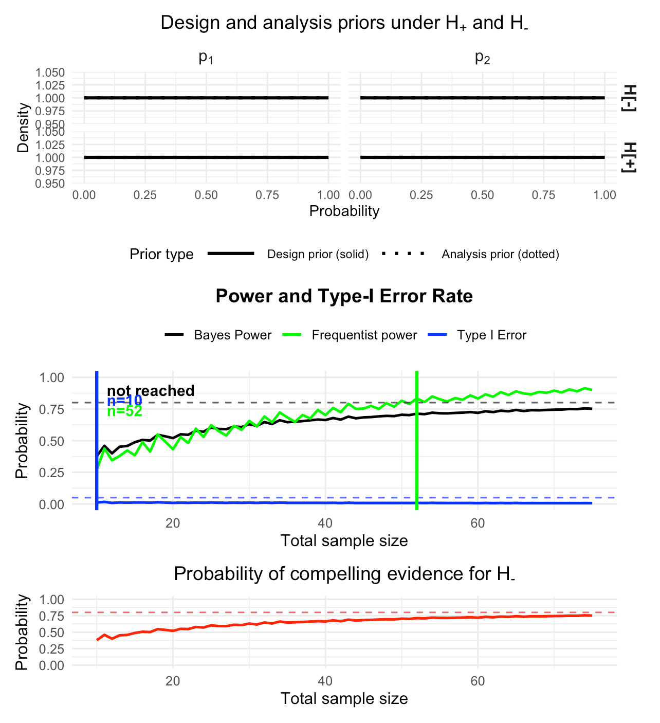

Figure 1: Visualization of the calibrated Bayesian two-arm one-stage phase II design with a binary endpoint

The summary and plot show that for the range of sample sizes provided to the function, under flat design priors, no sample size satisfies the requirement of Bayesian power $\geq 0.80$. Thus, if we want to obtain a calibrated design we can either increase n_max or choose more informative design priors. Alternatively, we could shift to a less stringent threshold for evidence $k$, e.g. $k=1/3$ instead of $k=1/10$, so it becomes easier for the Bayes factor to accumulate evidence in favour of $H_+$.

The arguments correspond closely to the conceptual requirements:

• k is the evidence threshold for rejecting the null (inverted Bayes factor). Here, k = 1/10 corresponds to moderately strong evidence against the null.
• k_f is the threshold for compelling evidence in favour of the null (here, $k_f = 10$ in favour of $H_-$).
• calibration selects which constraints to enforce: "Bayesian" uses Bayesian power, type-I error, and CE(H0); "frequentist", "hybrid", and "full" add frequentist constraints. Frequentist calibration implies that frequentist power and type-I-error rare calibrated, hybrid calibration implies that Bayesian power and frequentist type-I-error are calibrated, and full calibration implies that both frequentist and Bayesian power and type-I-error are calibrated.
• target_power, target_type1, and target_ce_h0 are the Bayesian calibration targets.
• p1_power and p2_power specify the assumed proportions for frequentist power (when used), here $p_1 = 0.3$ and $p_2 = 0.6$.
• alloc1 and alloc2 specify randomisation probabilities for control and treatment; here we use equal allocation.

The resulting object des shows in its print and summary output whether a feasible design was found and, if so, which sample sizes and operating characteristics are selected. The old three-panel plot is now available via

plot(des, type = "old")

which reproduces the original ntwoarmbinbf01(output = "plot") visualisation. For this default plot, it is also possible to just call

plot(des)

In addition, two more compact plot types are provided:

plot(des, type = "oc")          # operating characteristics across n_total
plot(des, type = "feasibility") # pointwise vs sustained feasibility across n_total

The old function ntwoarmbinbf01() is still available for backward compatibility. It now returns the same design object as design_twoarm_onestage_bf() and internally calls that function. A simple compatibility call is:

des_legacy <- ntwoarmbinbf01(
  k = 1/10, k_f = 10,
  power = 0.8, alpha = 0.05, pce_H0 = 0.8,
  test = "BF+-",
  nrange = c(10, 75), n_step = 1,
  progress = FALSE,
  compute_freq_t1e = TRUE,
  p1_power = 0.3, p2_power = 0.6,
  alloc1 = 0.5, alloc2 = 0.5,
  output = "numeric"
)

We plot the results:

plot(des_legacy, type = "old")

Figure 2: Visualization of the calibrated Bayesian two-arm one-stage phase II design with a binary endpoint

This code path is mainly intended for users with existing scripts; new analyses should use design_twoarm_onestage_bf() directly.

4. Informative design priors

The example above used flat design priors, which might be unrealistic in a variety of settings. While it would be possible to increase the maximum sample size n_max in the search range to eventually find a calibrated trial design, a more helpful approach is to use informative design priors. Such design priors should reflect the expectations investigators have about the effect of a novel drug or treatment. In particular, it is strongly recommended to use at least slightly informative design priors, because if no expectation about the effect of the drug or treatment (e.g. due to prior phase I trials) is made, this might be unrealistic from a practical point of view. Not only is the question why and whether a phase II trial should be conducted in such a case. Using flat design priors is highly unrealistic in several aspects:

• Suppose flat design priors are assumed under $H_1$ for the treatment and the control group. We focus on the treatment group just for a moment. All parameter values inside the unit interval $[0,1]$ are being assigned the same prior probability density value. As a consequence, all parameter values (or small regions around them, as from a measure theoretic-point of view single parameter values have prior probability of exactly zero) are equally likely a priori before any data are observed. This implies, that e.g. success probabilities like $p_2=0.99$ are equally likely a priori as $p_2=0.4$, which in almost all phase II trials would be a very questionable assumption for the treatment group in the two-arm setting.
• Using flat design priors under both $H_0$ and $H_1$ implies that when the null hypothesis is true and $p_1\leq p_2$ holds, all parameter values $p_1$ (the success probability in the control group) less than or equal to $p_2$ are equally likely a priori. However, in most phase II trials investigators would argue that extremely large differences $p_1 \leq p_2 \Leftrightarrow p_2-p_1 \geq 0$ in the success probabilities between both trial arms are less likely a priori than smaller ones. As a consequence, a more informative design prior under $H_0$ which places more mass at the boundary region $p_1=p_2$ could be more realistic.

Next, we therefore perform a sample size search for the ICT-107-type trial (balanced arms) under informative design priors with very strong evidence thresholds k = 1/30 and k_f = 30. Notice the additionally specified parameters a_1_d = 1, b_1_d = 2 and a_2_d = 2, b_2_d = 1 which are the design prior hyperparameters of the Beta design priors for $p_1$ and $p_2$ under $H_+$. These express slight optimism about the treatment effect in the sense that they can be thought of as having already observed 1 success and 2 failures in the control group and 2 successes and 1 failure in the treatment group. Also, we lower our requirements for the probability of compelling evidence in favour of $H_0$ to, say, $60$. We additionally require the reporting of the frequentist type-I-error for the calibrated design by specifying report_freq_type1 = TRUE in the function call:

des_informative <- design_twoarm_onestage_bf(
  n_min = 10,
  n_max = 100,
  k = 1/30,
  k_f = 30,
  test = "BF+-",
  calibration = "Bayesian",
  target_power = 0.80,
  target_type1 = 0.05,
  target_ce_h0 = 0.60,
  # design and analysis priors: flat Beta(1,1) everywhere
  a_0_d = 1, b_0_d = 1,
  a_0_a = 1, b_0_a = 1,
  a_1_d = 1, b_1_d = 2,
  a_2_d = 2, b_2_d = 1,
  a_1_a = 1, b_1_a = 1,
  a_2_a = 1, b_2_a = 1,
  # assumed true proportions for frequentist power (optional here)
  p1_power = 0.3, p2_power = 0.6,
  # report frequentist type-I-error? (optional here)
  report_freq_type1 = TRUE,
  # equal randomisation
  alloc1 = 0.5,
  alloc2 = 0.5,
  # require sustained feasibility over the next 10 larger n
  sustain_n = 10L,
  progress = FALSE
)

We summarize the results:

summary(des_informative)

Summary: One-stage two-arm Bayes factor design
---------------------------------------------
Mode:        optimal
Status:      Smallest feasible one-stage two-arm design found.
Calibration: Bayesian
Feasible:    yes

Search overview
  n evaluated          = 91
  pointwise feasible   = 28
  sustained feasible   = 27
  first pointwise n    = 72
  first sustained n    = 74

Selected design
  n_total = 74, n1 = 37, n2 = 37

The output shows that the first feasible sample size for which the target constraints hold was $n=72$. However, as we require the next ten sample sizes for the operating characteristics not to violate their respective constraint (that is, power should not decrease below its specified target threshold, type-I-error not increase above its specified target threshold and probability of compelling evidence not drop below its specified target threshold for the next ten observations), the first sample size for which this holds is $n=74$. This leads to the selected design with $n_1=37$ and $n_2=37$ patients in the control and treatment group.

Details on the implementation: For each operating characteristic we also compute a metric‑specific sustained attainment sample size that respects the user‑supplied sustain_n constraint. Concretely, we form separate logical indicators over the search grid for Bayesian power (≥ target_power), Bayesian type‑I error (≤target_type1), CE(H0) (≥target_ce_h0), and frequentist power (≥target_freq_power). Given such an indicator vector for a particular metric, we then search for the first total sample size $n$ such that the metric’s target is satisfied not only at $n$, but also for all subsequent total sample sizes in the forward window of length sustain_n + 1, truncated at the upper end of the search range. The vertical reference lines in the diagnostic plots are drawn at these metric‑specific sustained crossing points. This ensures that the plotted “required” sample sizes reflect the same sustained feasibility logic as the calibration itself, so that, for example, Bayesian power may first reach its nominal threshold at $n=72$, but the corresponding vertical line will only be shown at $n=74$ if the power constraint fails to remain satisfied over the next sustain_n total sample sizes.

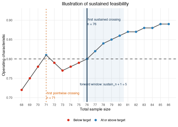The above figure illustrates the sustained feasibility logic which currently is implemented in the calibration algorithm. For $n=71$ in this toy example, and sustain_n + 1 = 5, even though the threshold of 80% is achieved, the sample size eventually selected is $n=76$. For $n=76$, the next $5$ sample sizes up to $n=80$ satisfy the operating characteristic threshold of at leat 80%, which is not the case for $n=71$.

Now, back to our calibrated design. We plot the results:

plot(des_informative)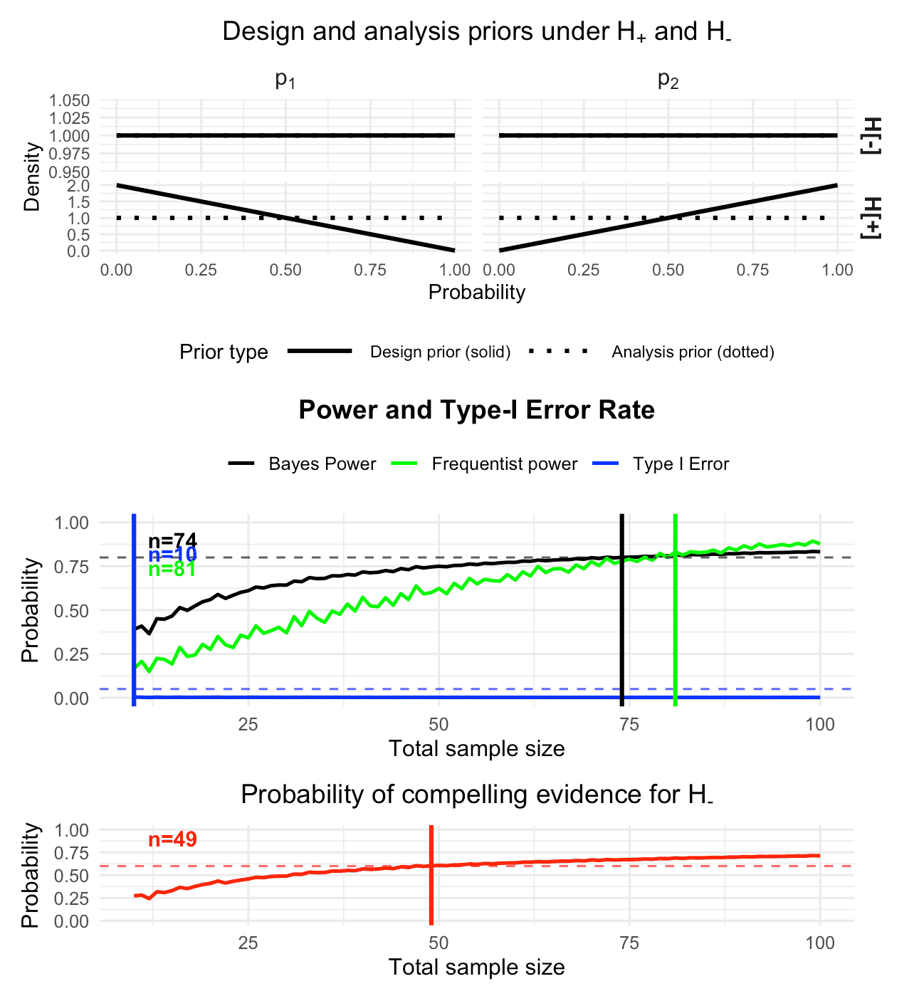

Figure 3: Visualization of the calibrated Bayesian two-arm one-stage phase II design with a binary endpoint, using informative design priors under the alternative hypothesis

We see that now the Bayesian power is calibrated for $n=74$ patients per trial arm and does not drop below the required 80% for at least the next ten sample sizes (it does not drop below the 80% for any sample size up to $n=100$, as can be verified by the plot). Frequentist power is calibrated for $n=81$ patients trial arm. The Bayesian type-I-error is already calibrated for $n=10$, requiring only $5$ patients per trial arm. Importantly, the frequentist type-I-error is also calibrated and is $0.034<0.05$, as can be inspected by

print(des_informative)

One-stage two-arm Bayes factor design
------------------------------------
Mode: optimal
Status: Smallest feasible one-stage two-arm design found.
Calibration: Bayesian
Optional freq. Type-I reporting: on
Design: n_total = 74, n1 = 37, n2 = 37

Operating characteristics
 Power = 0.8004
 Type-I error = 0.0021
 CE(H0) = 0.6697
 Freq. Type-I = 0.0340
 Freq. Power = 0.7778

The probability of compelling evidence for $H_-$ is shown in the bottom plot. It is calibrated for $n=49$, so the trial design is fully calibrated from a Bayesian perspective if $n=74$ patients are recruited in total ($n_1=37$ in the control and $n_2=37$ in the treatment group). Then, the probability of compelling evidence is also calibrated.

Based on the above plot we can see that the probability of compelling evidence does not reach 80% in the sample size range up to $n=100$ patients. However, suppose we want a trial design which achieves such a high probability of compelling evidence for $H_0$, but we cannot afford to recruit more than $n=100$ patients in total. A possible solution is to modify the design priors under $H_-$ to express more information about our expectation of the effect the novel drug or treatment has.

Thus, we perform a sample size search for new ICT-107-type trial (balanced arms) under informative design priors with very strong evidence thresholds, and change the design prior under H- to achieve the target probability of compelling evidence PCE(H0) for even smaller sample sizes. Note that now, additionally, the design prior hyperparameters of the Beta design priors for $p_1$ and $p_2$ under $H_-$ are specified in a_1_d_Hminus = 2, b_1_d_Hminus = 1 and a_2_d_Hminus = 1, b_2_d_Hminus = 2. Note that we increased target_ce_h0 = 60 to target_ce_h0 = 0.80:

des_informative_higher_ce <- design_twoarm_onestage_bf(
  n_min = 10,
  n_max = 100,
  k = 1/30,
  k_f = 30,
  test = "BF+-",
  calibration = "Bayesian",
  target_power = 0.80,
  target_type1 = 0.05,
  target_ce_h0 = 0.80,
  # design and analysis priors: flat Beta(1,1) everywhere
  a_0_d = 1, b_0_d = 1,
  a_0_a = 1, b_0_a = 1,
  a_1_d = 1, b_1_d = 2,
  a_2_d = 2, b_2_d = 1,
  a_1_a = 1, b_1_a = 1,
  a_2_a = 1, b_2_a = 1,
  # design prior parameters under H_-
  a_1_d_Hminus = 2, b_1_d_Hminus = 1,
  a_2_d_Hminus = 1, b_2_d_Hminus = 2,
  # assumed true proportions for frequentist power (optional here)
  p1_power = 0.3, p2_power = 0.6,
  # report frequentist type-I-error? (optional here)
  report_freq_type1 = TRUE,
  # equal randomisation
  alloc1 = 0.5,
  alloc2 = 0.5,
  # require sustained feasibility over the next 10 larger n
  sustain_n = 10L,
  progress = FALSE
)

We check the results:

summary(des_informative_higher_ce)

Summary: One-stage two-arm Bayes factor design
---------------------------------------------
Mode:        optimal
Status:      Smallest feasible one-stage two-arm design found.
Calibration: Bayesian
Feasible:    yes

Search overview
  n evaluated          = 91
  pointwise feasible   = 28
  sustained feasible   = 27
  first pointwise n    = 72
  first sustained n    = 74

Selected design
  n_total = 74, n1 = 37, n2 = 37

The design has not changed. Why is that? We plot the results:

plot(des_informative_higher_ce)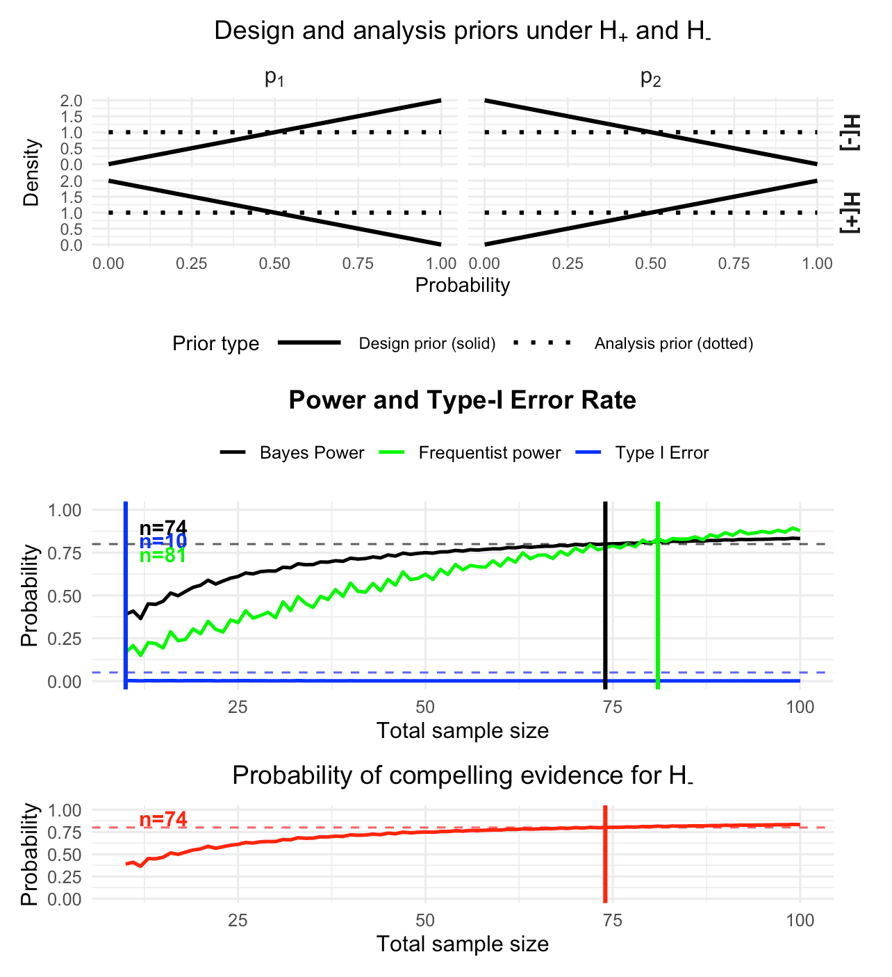

Figure 4: Visualization of the calibrated Bayesian two-arm one-stage phase II design with a binary endpoint, using informative design priors under both hypotheses and a stronger requirement on the probability of compelling evidence (80% instead of only 60%)

The plot shows that the calibration sample sizes for Bayesian power, type-I-error and frequentist power remain identical to the previous function call. The only thing which changed are the design priors under $H_-$ in the top panel, and the bottom panel for the probability of compelling evidence. First, the design priors under $H_-:p_2 \leq p_1$ have a form which puts more prior probability mass to small success probabilities in the treatment group with parameter $p_2$, and more prior probability mass to large success probabilities in the control group with parameter $p_1$. This is precisely expressed by $H_-:p_2 \leq p_1$, and thus under $H_0$, we can expect that evidence for $H_0$ accumulates faster. This is reflected in the bottom panel for the probability of compelling evidence, as now $n=74$ patients suffice to reach 80% probability of compelling evidence for $H_0$.

The result is a fully calibrated Bayesian design which meets Bayesian power demands of 80%, Bayesian type-I-error rate requirements of less than 5%, and our requirement of 80% on the probability of compelling evidence for $H_0$ (that is, $H_-$ in this case).

What about the frequentist operating characteristics of this design? We see that $n=81$ patients in total suffice to calibrate the design additionally in terms of frequentist power.

print(des_informative_higher_ce)

One-stage two-arm Bayes factor design
------------------------------------
Mode: optimal
Status: Smallest feasible one-stage two-arm design found.
Calibration: Bayesian
Optional freq. Type-I reporting: on
Design: n_total = 74, n1 = 37, n2 = 37

Operating characteristics
 Power = 0.8004
 Type-I error = 0.0011
 CE(H0) = 0.8004
 Freq. Type-I = 0.0340
 Freq. Power = 0.7778

The type-I-error is still calibrated, so choosing $n=81$ patients in total even yields a fully calibrated design both from a Bayesian and frequentist perspective.

The calibration function design_twoarm_onestage_bf reveals several aspects. If a balanced design with equal randomization probabilities is desired, then:

• n=81 patients in total (41 patients per trial arm) are needed for 80% frequentist power at ICT-107 effect size when evidence threshold $k=1/30$ is used. Here, the assumption is that the true proportions are $p_1=0.3$ and $p_2=0.6$, which can easily be modified if a more optimistic or pessimistic assumption is warranted
• n=74 patients in total (37 patients per trial arm) are needed for 80% Bayesian power at ICT-107 effect size when evidence threshold $k=1/30$ is used, and slightly informative Beta design priors are assumed under $H_+$.
• Type-I error control both from a frequentist perspective (≤5% across designs when $k=1/30$ is used) and from a Bayesian perspective, where for the latter only $n=10$ patients in total (5 patients per trial arm) are required.
• High P(CE|H-) guarantees that under $H_-$ there is 80% probability to find a Bayes factor of at least $k_f=30$ in favour of $H_-$. n=74 patients in total (37 patients per trial arm) are required to assert this probability of compelling evidence for $H_-$.

5. Unequal randomization probabilities

In the original ICT-107 trial, $2/3$ of the patients was randomized into the treatment group, while $1/3$ of the patients was randomized into the control group. We can use the parameters alloc1 and alloc2 to specify randomization probabilities for the control and treatment arms and carry out the Bayesian sample size calculations based on these randomization probabilities. As an example, we rerun the last calibration, but use the randomization probabilities of the ICT-107 trial:

des_informative_higher_ce_uneq_alloc <- design_twoarm_onestage_bf(
  n_min = 10,
  n_max = 100,
  k = 1/30,
  k_f = 30,
  test = "BF+-",
  calibration = "Bayesian",
  target_power = 0.80,
  target_type1 = 0.05,
  target_ce_h0 = 0.80,
  # design and analysis priors: flat Beta(1,1) everywhere
  a_0_d = 1, b_0_d = 1,
  a_0_a = 1, b_0_a = 1,
  a_1_d = 1, b_1_d = 2,
  a_2_d = 2, b_2_d = 1,
  a_1_a = 1, b_1_a = 1,
  a_2_a = 1, b_2_a = 1,
  # design prior parameters under H_-
  a_1_d_Hminus = 2, b_1_d_Hminus = 1,
  a_2_d_Hminus = 1, b_2_d_Hminus = 2,
  # assumed true proportions for frequentist power (optional here)
  p1_power = 0.3, p2_power = 0.6,
  # report frequentist type-I-error? (optional here)
  report_freq_type1 = TRUE,
  # equal randomisation
  alloc1 = 1/3,
  alloc2 = 2/3,
  # require sustained feasibility over the next 10 larger n
  sustain_n = 10L,
  progress = FALSE
)

We summarize the results:

summary(des_informative_higher_ce_uneq_alloc)

Summary: One-stage two-arm Bayes factor design
---------------------------------------------
Mode:        optimal
Status:      Smallest feasible one-stage two-arm design found.
Calibration: Bayesian
Feasible:    yes

Search overview
  n evaluated          = 91
  pointwise feasible   = 18
  sustained feasible   = 18
  first pointwise n    = 83
  first sustained n    = 83

Selected design
  n_total = 83, n1 = 28, n2 = 55

We plot the results:

plot(des_informative_higher_ce_uneq_alloc)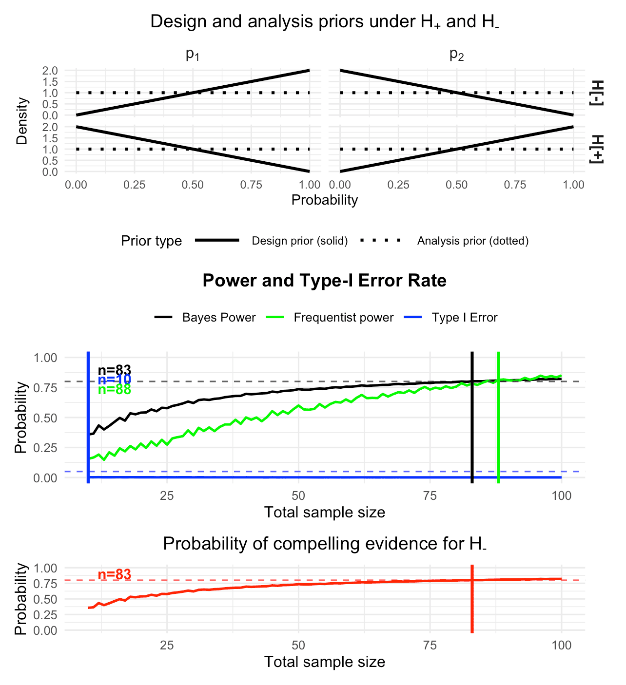

Figure 5: Visualization of the calibrated Bayesian two-arm one-stage phase II design with a binary endpoint, using informative design priors under both hypotheses and a stronger requirement on the probability of compelling evidence (80% instead of only 60%). Additionally, unequal randomization probabilities are used when calibrating the design.

Remember that the sample size shown at the x-axis in the power and type-I-error rate plot as well as in the probability of compelling evidence plot is the total sample size in both arms. We see that now we need $n=83$ patients in total to reach Bayesian power of 80%, while $n=88$ patients in total are required for frequentist power calibration of 80%. The probability of compelling evidence reaches 80% at $n=83$ patients in total. The frequentist type-I-error rate is still below the required 5% threshold, too:

print(des_informative_higher_ce_uneq_alloc)

One-stage two-arm Bayes factor design
------------------------------------
Mode: optimal
Status: Smallest feasible one-stage two-arm design found.
Calibration: Bayesian
Optional freq. Type-I reporting: on
Design: n_total = 83, n1 = 28, n2 = 55

Operating characteristics
 Power = 0.8018
 Type-I error = 0.0011
 CE(H0) = 0.8018
 Freq. Type-I = 0.0369
 Freq. Power = 0.7829

6. Design Recommendations based on the calibration

If the original 2:1 randomization of the ICT-107 trial is used and two thirds of the patients are randomized into the treatment group, then:

• n=83 patients in total (28 patients in the control arm and 55 in the treatment arm) are needed for 80% Bayesian power at ICT-107 effect size when evidence threshold $k=1/30$ is used, and slightly informative Beta design priors are assumed under $H_+$.
• Type-I error control both from a frequentist perspective (≤5% across designs when $k=1/30$ is used) and from a Bayesian perspective, where for the latter only $n=10$ patients in total (both arms) are required.
• High P(CE|H-) guarantees that under $H_-$ there is 80% probability to find a Bayes factor of at least $k_f=30$ in favour of $H_-$. n=83 patients in total (28 in the control arm and 55 in the treatment arm) are required to assert this probability of compelling evidence for $H_-$.
• n=88 patients in total (29 patients in the control arm and 59 in the treatment arm) are needed for 80% frequentist power at ICT-107 effect size when evidence threshold $k=1/30$ is used. Here, the assumption is that the true proportions are $p_1=0.3$ and $p_2=0.6$, which can easily be modified if a more optimistic or pessimistic assumption is warranted

To fulfill all four requirements, it thus suffices if $n_1=29$ patients in the control arm and $n_2=59$ in the treatment arm are enrolled in the trial, and the Bayes factor thresholds $k=1/30$ and $k_f=30$ are used for decision making about the hypotheses $H_+$ and $H_-$ under consideration.

For a Bayesian calibration only, it suffices if $n_1=28$ patients in the control arm and $n_2=55$ in the treatment arm are enrolled in the trial.

Summary

This vignette has illustrated how to design and calibrate two‑arm one‑stage Bayes factor trials with binary endpoints using the bfbin2arm package. The core workflow starts from specifying a Bayes factor test (two‑sided or directional), choosing coherent design and analysis priors under the competing hypotheses, and then mapping clinical requirements onto calibration targets for Bayesian power, Bayesian type‑I error, and the Bayesian probability of compelling evidence for the null (or $H_-$ in directional tests). The central calibration function design_twoarm_onestage_bf() searches over a user‑defined grid of total sample sizes and returns a design object that contains the selected allocation $(n_1, n_2)$, the corresponding total sample size $n_{\text{total}}$, and both Bayesian and frequentist operating characteristics at the chosen design.

A key innovation is the use of a sustained feasibility constraint, controlled by the argument sustain_n, which guards against oscillatory behaviour of operating characteristics driven by the discreteness of the binomial model. Instead of treating a sample size as feasible as soon as it meets its calibration thresholds pointwise, the algorithm only accepts a candidate $n_{\text{total}}$ if all relevant targets hold at that $n_{\text{total}}$ and continue to hold for at least the next sustain_n larger total sample sizes within the search range. The diagnostic plots reflect this logic: for each operating characteristic (Bayesian power, Bayesian type‑I error, CE(H0), and optional frequentist power), the vertical reference line is drawn at the first total sample size where the corresponding metric attains its target in this sustained sense. As a result, the graphical summaries and numerical design recommendations are aligned and directly interpretable as robust to local oscillations in the operating characteristic curves.

Using the ICT‑107 phase II trial as a running example, we have shown how flat design priors can be replaced by more informative priors that encode realistic expectations about treatment and control response rates. This shift often allows one (1) to achieve the desired calibration targets at substantially smaller total sample sizes compared to flat priors and (2) achieve higher constraints on certain operating characteristics such as the probability of compelling evidence for identical sample sizes, especially when strong evidence thresholds (e.g. $k = 1/30$, $k_f = 30$) are required. The vignette has also demonstrated how to handle equal and unequal randomization, how to request frequentist type‑I error and power alongside the Bayesian criteria, and how to interpret the resulting design recommendations in terms of total sample size $n_{\text{total}}$ and arm‑specific allocations. Overall, the bfbin2arm package provides a flexible, unified framework in which Bayesian, frequentist, hybrid, and fully dual calibrations can be performed and visualised in a way that is directly tied to clinically meaningful decision thresholds.

Further details on the methodology can be found in (Kelter 2026).

References

Kelter, Riko. 2026. Power and Sample Size Calculations for Bayes Factors in Two-Arm Clinical Phase II Trials with Binary Endpoints. https://arxiv.org/abs/2603.01715.

Wen, Patrick Y., David A. Reardon, Terri S. Armstrong, et al. 2019. “A Randomized Double-Blind Placebo-Controlled Phase II Trial of Dendritic Cell Vaccine ICT-107 in Newly Diagnosed Patients with Glioblastoma.” Clinical Cancer Research: An Official Journal of the American Association for Cancer Research 25 (19): 5799–807. https://doi.org/10.1158/1078-0432.CCR-19-0261.