Calibration of Bayesian one-stage designs for single-arm phase II trials with binary endpoints

Riko Kelter
Institute of Medical Statistics and Computational Biology
Faculty of Medicine, University of Cologne
Cologne, Germany

23 June 2026

Introduction

This vignette illustrates how to calibrate a one-stage single-arm Bayes factor design for a binary endpoint. The goal is to determine the smallest total sample size that satisfies pre-specified Bayesian and/or frequentist operating characteristics. The underlying statistical theory is developed in (Kelter and Pawel 2025a), extended to the single-arm two-stage optimal setting in (Kelter and Pawel 2025b), and further developed to the two-arm single-stage setting in (Kelter 2026).

How to design a Bayesian trial: Overview of the calibration algorithm

The workflow implemented in the package follows the fixed-sample Bayes factor calibration framework proposed in Kelter and Pawel (2025a): Choose design and analysis priors, specify an evidence threshold on the scale, compute operating characteristics as a function of the sample size, and select the smallest feasible design.

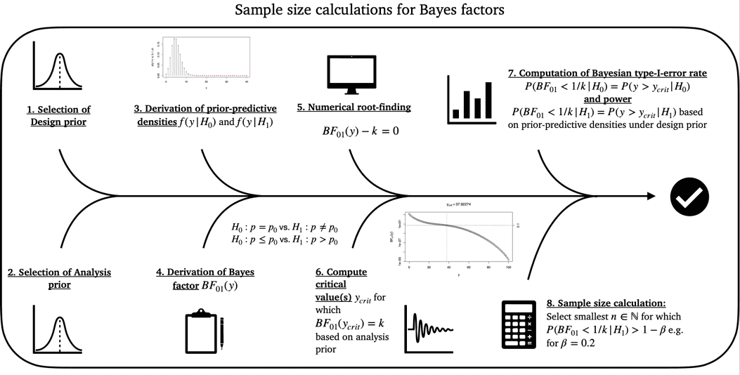
Figure 1: Illustration of the calibration algorithm for an optimal Bayesian single-arm phase II design with a binary endpoint

Figure 1 visualizes the calibration methodology in detail. Based on the selected design and analysis priors, the prior predictive and the Bayes factor, the critical value $y_{crit}$ is found via numerical root finding (step 5. and 6. in Figure 1). Based on this critical value, in the single-arm setting, the relationship

$$P(BF_{01}<1/k|H_i)=P(y>y_{crit}|H_i)$$

holds for both hypotheses $H_i$, $i\in \{0,1\}$. When $i=0$, this implies one can easily calculate the Bayesian type-I-error rate as

$$P(BF_{01}<1/k|H_0)=P(y>y_{crit}|H_0)$$

while for $i=1$, the latter becomes the Bayesian power:

$$P(BF_{01}<1/k|H_1)=P(y>y_{crit}|H_1)$$

For specified target constraints $\alpha \in (0,1)$ and $\beta \in (0,1)$, one can then calculate the smallest $n\in \mathbb{N}$, for which $$P(BF_{01}<1/k|H_0)=P(y>y_{crit}|H_0)\leq \alpha$$ and

$$P(BF_{01}<1/k|H_1)=P(y>y_{crit}|H_1)> 1-\beta$$

A further metric for calibration is the probability of compelling evidence

$$P(BF_{01}>k_f|H_0)$$

which can likewise be calibrated to achieve at least a threshold $f\in (0,1)$. Here, the event $BF_{01}>k_f$ can be interpreted as the Bayes factor providing sufficient evidence $k_f >0$ in favour of $H_0$, when $H_0$ is indeed true. If this probability is calibrated, additionally to Bayesian type-I-error rate and power, one can be certain when the trial is carried out, the event $BF_{01}>k_f$ is reached with probability $f$ when $H_0$ indeed holds. Thus, when the null hypothesis is true we will often find sufficient evidence to really accept $H_0$ instead of remaining indecisive about whether $H_0$ or $H_1$ is true.

---

Basic calibration

We consider a phase II setting with null response probability p0 = 0.2 and an efficacy threshold k = 1/3 on the scale. We assume slightly optimistic design priors via da1 = 2.5 and db1 = 2 under $H_1$, a flat design prior under $H_0$, specified via da0 = 1 and db0 = 1, and flat analysis priors under both $H_0$ and $H_1$ (specified via a0 = 1, b0 = 1, a1 = 1 and b1 = 1). We test the hypotheses

$$H_0:p\leq 0.2 \text{ versus } H_1:p>0.2$$

against each other, so we use the argument type = "direction" and set p0 = 0.2. We limit the sample size range to the minimum and maximum values n_min = 10 and n_max = 200, and require 80% Bayesian power, specified via target_power = 0.80. Also, we require a Bayesian type-I-error rate of 5% or less, specified via the argument target_type1 = 0.05:

des_bayes <- design_singlearm_onestage_bf(
  n_min = 10,
  n_max = 200,
  k = 1/3,
  p0 = 0.2,
  a0 = 1, b0 = 1,
  a1 = 1, b1 = 1,
  da0 = 1, db0 = 1,
  da1 = 2.5, db1 = 2,
  type = "direction",
  calibration = "Bayesian",
  target_power = 0.8,
  target_type1 = 0.05
)

We can inspect the results as follows:

summary(des_bayes)
#> Summary: One-stage single-arm Bayes factor design
#> ------------------------------------------------
#> Calibration: Bayesian 
#> Sustain:  10  future n
#> Feasible   : TRUE 
#> Status     : Smallest feasible one-stage design found. 
#> 
#> Selected design
#>   n          : 13 
#>   k          : 0.333 
#> 
#> Operating characteristics
#>   Bayes power      : 0.821 
#>   Bayes type-I     : 0.021 
#>   CE(H0)           :   NA 
#>   Freq power       :   NA 
#>   Freq type-I      : 0.099

Operating-characteristic curves

The search results can be visualized directly.

plot(des_bayes)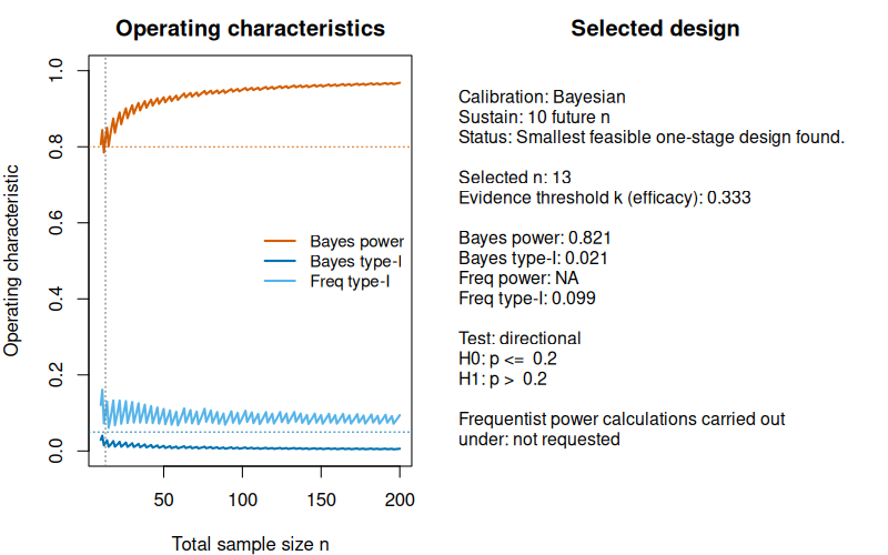

The left panel shows Bayesian power and type-I error, together with optional frequentist overlays if a point alternative is supplied.

The right panel showsthe relevant operating characteristics of the trial design isolated by the calibration algorithm. In this case, no frequentist power calculations were required, so the frequentist power is shown as NA (not available), and the lower part states that frequentist power calculations under a point alternative were not requested. We can quickly see that Bayesian power and type-I-error rate are calibrated for $n=13$ already, so when choosing the evidence threshold $k=1/3$, $n=13$ patients suffice to yield a calibrated Bayesian design. Also, the output shows that this design is not calibrated in terms of the frequentist type-I-error rate, which is computed via a grid-search and in this case is $9.9\%$.

Note that the beta-binomial model induces the zig-zag shape of the resulting curves for the operating characteristics such as power and type-I-error rate. As a consequence, the calibration algorithm by default requires the power not to drop below the specified target threshold for the next ten sample sizes. This is also customisably via the parameter sustain_n, which is also shown in the summary output above in form of the text “Sustain: 10 future n”.

Adding a constraint on the probability of compelling evidence

Next, we could add a constraint on the probability of compelling evidence for $H_0$. An optional CE(H0) constraint can be imposed through target_ce_h0. This is useful when one also wants the design to have a sufficient probability of yielding compelling evidence in favour of the null hypothesis

$$P(BF_01>k_f|H_0)>f$$

for some $f\in (0,1)$ and futility evidence threshold $k_f>1$. Now, we use $f=0.60$ and $k_f=3$, specified via the arguments target_ce_h0 = 0.60 and k_ce = 3. Everything else remains the same, but we also add the argument dp = 0.4 to compute frequentist power under the point alternative $p=0.4$:

des_bayes_ce <- design_singlearm_onestage_bf(
  n_min = 10,
  n_max = 200,
  k = 1/3,
  p0 = 0.2,
  a0 = 1, b0 = 1,
  a1 = 1, b1 = 1,
  da0 = 1, db0 = 1,
  da1 = 2.5, db1 = 2,
  type = "direction",
  calibration = "Bayesian",
  target_power = 0.8,
  target_type1 = 0.05,
  target_ce_h0 = 0.6,
  k_ce = 3,
  dp = 0.4
)

We inspect the results:

summary(des_bayes_ce)
#> Summary: One-stage single-arm Bayes factor design
#> ------------------------------------------------
#> Calibration: Bayesian 
#> Sustain:  10  future n
#> Feasible   : FALSE 
#> Status     : No feasible one-stage design found.

Now, no design could be found which fulfills our target constraints. Before we see why, note that since we added the parameter dp = 0.4 to the above function call frequentist power is additionally calculated under the point alternative $p=0.4$ in the single-arm case. We can always add this to a design calibration, but the calibration mode (specified via the argument calibration) decides which metric is the benchmark for finding a feasible design (that is, a sufficiently large sample size to meet our specified target constraints). Thus, frequentist power is calculated here solely post-hoc for the calibrated design. The calibrated design itself is calibrated according to the Bayesian target power and type-I-error rate.

We can plot the resulting design:

plot(des_bayes_ce)

The plot shows that the factor which causes problems is the probability of compelling evidence. In the sample size range up to $n=200$, it stays below the required 60%, so no calibrated design can be found. If we lower the requirement to, say, 50%, we get:

des_bayes_ce50 <- design_singlearm_onestage_bf(
  n_min = 10,
  n_max = 200,
  k = 1/3,
  p0 = 0.2,
  a0 = 1, b0 = 1,
  a1 = 1, b1 = 1,
  da0 = 1, db0 = 1,
  da1 = 2.5, db1 = 2,
  type = "direction",
  calibration = "Bayesian",
  target_power = 0.8,
  target_type1 = 0.05,
  target_ce_h0 = 0.5,
  k_ce = 3,
  dp = 0.4
)

We inspect the fit:

summary(des_bayes_ce50)
#> Summary: One-stage single-arm Bayes factor design
#> ------------------------------------------------
#> Calibration: Bayesian 
#> Sustain:  10  future n
#> Feasible   : TRUE 
#> Status     : Smallest feasible one-stage design found. 
#> 
#> Selected design
#>   n          : 65 
#>   k          : 0.333 
#>   k_ce       :    3 
#> 
#> Operating characteristics
#>   Bayes power      : 0.934 
#>   Bayes type-I     : 0.009 
#>   CE(H0)           : 0.574 
#>   Freq power       : 0.986 
#>   Freq type-I      : 0.085

We can plot the resulting design:

plot(des_bayes_ce50)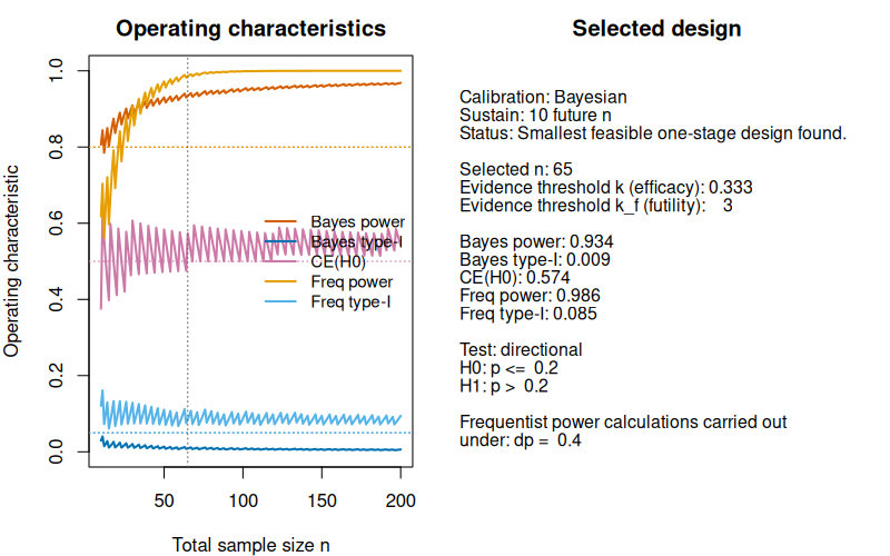

Now a calibrated design can be found, as expected.

Full Bayes-frequentist calibration

The same interface also supports frequentist and fully joint calibration modes. We change calibration = "Bayesian" to calibration = "full", and specify our target constraints for frequentist power and type-I-error rate via the arguments target_freq_power = 0.8 and target_freq_type1 = 0.05.

des_full <- design_singlearm_onestage_bf(
  n_min = 10,
  n_max = 100,
  k = 1/3,
  p0 = 0.2,
  a0 = 1, b0 = 1,
  a1 = 1, b1 = 1,
  dp = 0.4,
  da0 = 1, db0 = 1,
  da1 = 2.5, db1 = 2,
  type = "direction",
  calibration = "full",
  target_power = 0.8,
  target_type1 = 0.05,
  target_freq_power = 0.8,
  target_freq_type1 = 0.05
)

summary(des_full)
#> Summary: One-stage single-arm Bayes factor design
#> ------------------------------------------------
#> Calibration: full 
#> Sustain:  10  future n
#> Feasible   : FALSE 
#> Status     : No feasible one-stage design found.

Now, given our priors and evidence thresholds no feasible one-stage design was found in the specified sample size range. We can see the reason for this by inspecting

head(des_full$search_results)
#>    n     power      type1 ce_h0 power_naive type1_naive erased_power
#> 1 10 0.8065237 0.02925913    NA   0.8065237  0.02925913            0
#> 2 11 0.8438969 0.04026381    NA   0.8438969  0.04026381            0
#> 3 12 0.7849683 0.01482212    NA   0.7849683  0.01482212            0
#> 4 13 0.8206335 0.02085515    NA   0.8206335  0.02085515            0
#> 5 14 0.8498421 0.02813328    NA   0.8498421  0.02813328            0
#> 6 15 0.8016997 0.01109326    NA   0.8016997  0.01109326            0
#>   erased_type1 freq_power freq_type1 freq_power_naive freq_type1_naive
#> 1            0  0.6177194 0.12087388        0.6177194       0.12087388
#> 2            0  0.7037157 0.16113920        0.7037157       0.16113920
#> 3            0  0.5618218 0.07255550        0.5618218       0.07255550
#> 4            0  0.6469582 0.09913061        0.6469582       0.09913061
#> 5            0  0.7207430 0.12983963        0.7207430       0.12983963
#> 6            0  0.5967844 0.06105143        0.5967844       0.06105143
#>   erased_freq_power erased_freq_type1 bayes_ok freq_ok hybrid_ok feasible_ce
#> 1                 0                 0     TRUE   FALSE     FALSE        TRUE
#> 2                 0                 0     TRUE   FALSE     FALSE        TRUE
#> 3                 0                 0    FALSE   FALSE     FALSE        TRUE
#> 4                 0                 0     TRUE   FALSE     FALSE        TRUE
#> 5                 0                 0     TRUE   FALSE     FALSE        TRUE
#> 6                 0                 0     TRUE   FALSE     FALSE        TRUE
#>   feasible_pointwise feasible calibration
#> 1              FALSE    FALSE        full
#> 2              FALSE    FALSE        full
#> 3              FALSE    FALSE        full
#> 4              FALSE    FALSE        full
#> 5              FALSE    FALSE        full
#> 6              FALSE    FALSE        full

We can quickly see that the frequentist type-I-error of all designs is simply too large:

range(des_full$search_results$freq_type1)
#> [1] 0.06105143 0.16113920

Increasing the evidence threshold $k$ leads to the situation that it becomes harder for the Bayes factor to accumulate evidence in favour of $H_1$, thus also decreasing the type-I-error rates (both the Bayesian and frequentist ones). Thus, we refit our design as follows by changing k = 1/3 to k = 1/10:

des_full_strong_ev <- design_singlearm_onestage_bf(
  n_min = 10,
  n_max = 100,
  k = 1/10,
  p0 = 0.2,
  a0 = 1, b0 = 1,
  a1 = 1, b1 = 1,
  dp = 0.4,
  da0 = 1, db0 = 1,
  da1 = 2.5, db1 = 2,
  type = "direction",
  calibration = "full",
  target_power = 0.8,
  target_type1 = 0.05,
  target_freq_power = 0.8,
  target_freq_type1 = 0.05
)

We investigate the fit:

summary(des_full_strong_ev)
#> Summary: One-stage single-arm Bayes factor design
#> ------------------------------------------------
#> Calibration: full 
#> Sustain:  10  future n
#> Feasible   : TRUE 
#> Status     : Smallest feasible one-stage design found. 
#> 
#> Selected design
#>   n          : 38 
#>   k          :  0.1 
#> 
#> Operating characteristics
#>   Bayes power      : 0.866 
#>   Bayes type-I     : 0.003 
#>   CE(H0)           :   NA 
#>   Freq power       : 0.814 
#>   Freq type-I      : 0.029

We plot the fit:

plot(des_full_strong_ev)

Frequentist calibration

We turn to frequentist calibration of our design, and build upon the fully calibrated design above. We change the calibration mode accordingly to frequentist:

des_freq_strong_ev <- design_singlearm_onestage_bf(
  n_min = 10,
  n_max = 100,
  k = 1/10,
  p0 = 0.2,
  a0 = 1, b0 = 1,
  a1 = 1, b1 = 1,
  dp = 0.4,
  da0 = 1, db0 = 1,
  da1 = 2.5, db1 = 2,
  type = "direction",
  calibration = "frequentist",
  target_power = 0.8,
  target_type1 = 0.05,
  target_freq_power = 0.8,
  target_freq_type1 = 0.05
)

summary(des_freq_strong_ev)
#> Summary: One-stage single-arm Bayes factor design
#> ------------------------------------------------
#> Calibration: frequentist 
#> Sustain:  10  future n
#> Feasible   : TRUE 
#> Status     : Smallest feasible one-stage design found. 
#> 
#> Selected design
#>   n          : 38 
#>   k          :  0.1 
#> 
#> Operating characteristics
#>   Bayes power      : 0.866 
#>   Bayes type-I     : 0.003 
#>   CE(H0)           :   NA 
#>   Freq power       : 0.814 
#>   Freq type-I      : 0.029

Note in the above call, that the arguments target_power = 0.8 and target_type1 = 0.05 could also be removed, as they play no role when the calibration parameter is set to frequentist. target_power and target_type1 only specify the target constraints for calibration modes which involve a Bayesian component like calibration = "Bayesian", calibration = "hybrid" or calibration = "full".

Based on the summary output we see that the design which is calibrated in terms of frequentist type-I-error and power is also fully calibrated. This can also be seen from the last plot, because the Bayesian type-I-error and power meet their respective target constraints for already smaller sample size. The limiting factor in the fully calibrated design thus is the frequentist power, which is only achieved for $n=38$ (see the left panel in the last plot above).

Hybrid calibration

An interesting alternative is hybrid calibration. We do not provide detailed information here, but the core idea is to report Bayesian power, which often is more realistic than frequentist power under a specific point alternative, and frequentist type-I-error. Thus, from a regulatory perspective, the frequentist type-I-error is often the limiting or hard factor that must be met, as it constitutes a worst-case scenario, but Bayesian power might be more realistic under a slightly informative design prior. We set the calibration mode to hybrid:

des_hybrid_strong_ev <- design_singlearm_onestage_bf(
  n_min = 10,
  n_max = 100,
  k = 1/10,
  p0 = 0.2,
  a0 = 1, b0 = 1,
  a1 = 1, b1 = 1,
  dp = 0.4,
  da0 = 1, db0 = 1,
  da1 = 2.5, db1 = 2,
  type = "direction",
  calibration = "hybrid",
  target_power = 0.8,
  target_type1 = 0.05,
  target_freq_power = 0.8,
  target_freq_type1 = 0.05
)

summary(des_hybrid_strong_ev)
#> Summary: One-stage single-arm Bayes factor design
#> ------------------------------------------------
#> Calibration: hybrid 
#> Sustain:  10  future n
#> Feasible   : TRUE 
#> Status     : Smallest feasible one-stage design found. 
#> 
#> Selected design
#>   n          : 23 
#>   k          :  0.1 
#> 
#> Operating characteristics
#>   Bayes power      : 0.809 
#>   Bayes type-I     : 0.004 
#>   CE(H0)           :   NA 
#>   Freq power       : 0.612 
#>   Freq type-I      : 0.027

We see that now the feasible sample size to calibrate our design has changed from $n=38$ to only $n=23$. Thus, the hybrid design required fewer patients.

plot(des_hybrid_strong_ev)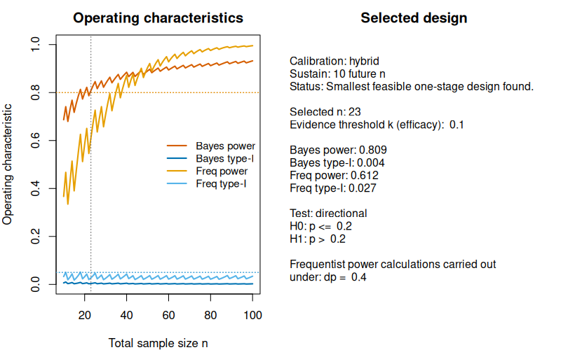

The plot clearly shows that Bayesian power is the limiting factor here: From $n=23$ patients on, it passes the required 80% threshold. Bayesian and frequentist type-I-error are controlled for even smaller sample sizes, and from our previous fully and frequentist calibration results we know that frequentist power achieves the required 80% target power only for $n=38$. Thus, shifting to a Bayesian notion of power under the slightly informative design priors under $H_1$ yields a reduction in sample size of $15$ patients, which is non-negligible.

We could also add a probability of compelling evidence constraint to that design by adding the arguments k_ce = 3 and target_ce_h0 = 0.60, indicating we require at least 60% probability of compelling evidence for $H_0$ based on a evidence threshold $k_f = 3$:

des_hybrid_strong_ev_with_ce <- design_singlearm_onestage_bf(
  n_min = 10,
  n_max = 100,
  k = 1/10,
  k_ce = 3,
  p0 = 0.2,
  a0 = 1, b0 = 1,
  a1 = 1, b1 = 1,
  dp = 0.4,
  da0 = 1, db0 = 1,
  da1 = 2.5, db1 = 2,
  type = "direction",
  calibration = "hybrid",
  target_power = 0.8,
  target_type1 = 0.05,
  target_ce_h0 = 0.6,
  target_freq_power = 0.8,
  target_freq_type1 = 0.05
)

summary(des_hybrid_strong_ev_with_ce)
#> Summary: One-stage single-arm Bayes factor design
#> ------------------------------------------------
#> Calibration: hybrid 
#> Sustain:  10  future n
#> Feasible   : FALSE 
#> Status     : No feasible one-stage design found.

We see that no calibrated design could be found in the sample size range specified. The following plot shows why:

plot(des_hybrid_strong_ev_with_ce)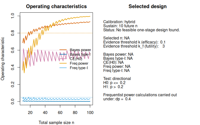

The probability of compelling evidence simply does not reach the target 60% in the specified sample size range. Thus, we could either increase that range by increasing n_max or adopting different design priors. Alternatively, we could lower our requirement on the probability of compelling evidence to, say, 50% as follows:

des_hybrid_strong_ev_with_ce50 <- design_singlearm_onestage_bf(
  n_min = 10,
  n_max = 100,
  k = 1/10,
  k_ce = 3,
  p0 = 0.2,
  a0 = 1, b0 = 1,
  a1 = 1, b1 = 1,
  dp = 0.4,
  da0 = 1, db0 = 1,
  da1 = 2.5, db1 = 2,
  type = "direction",
  calibration = "hybrid",
  target_power = 0.8,
  target_type1 = 0.05,
  target_ce_h0 = 0.5,
  target_freq_power = 0.8,
  target_freq_type1 = 0.05
)

summary(des_hybrid_strong_ev_with_ce50)
#> Summary: One-stage single-arm Bayes factor design
#> ------------------------------------------------
#> Calibration: hybrid 
#> Sustain:  10  future n
#> Feasible   : TRUE 
#> Status     : Smallest feasible one-stage design found. 
#> 
#> Selected design
#>   n          : 65 
#>   k          :  0.1 
#>   k_ce       :    3 
#> 
#> Operating characteristics
#>   Bayes power      : 0.904 
#>   Bayes type-I     : 0.002 
#>   CE(H0)           : 0.574 
#>   Freq power       : 0.952 
#>   Freq type-I      : 0.026

plot(des_hybrid_strong_ev_with_ce50)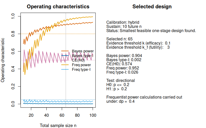

Relationship to the two-stage design

The one-stage design can be viewed as the fixed-sample baseline. In the package, the function design_singlearm_bf() extends this framework to a two-stage design with one interim analysis and early stopping for futility.

Summary

In this vignette we demonstrated how to calibrate one-stage single-arm Bayes factor designs for phase II trials with binary endpoints using the functions provided in the bfbin2arm package. The calibration framework combines design and analysis priors, Bayes-factor evidence thresholds, and target operating characteristics into a fully numerical search over the total sample size. Within this framework, users can work in purely Bayesian, purely frequentist, or hybrid modes, and optionally impose an additional constraint on the probability of compelling evidence in favour of the null hypothesis.

We illustrated how to obtain the smallest feasible design under Bayesian calibration, and how to visualize the resulting operating-characteristic curves via the dedicated plotting method. We also showed how to extend the calibration by adding a probability of compelling evidence (CE) constraint, and how the chosen futility threshold $k_f$ (the parameter k_ce) and the target level for the probability of compelling evidence interact with the achievable power and type-I error in a given sample size range. Finally, we discussed the sustain parameter sustain_n, which requires that the chosen design remains feasible for a number of larger sample sizes and thus guards against local beta–binomial oscillations in the operating characteristics.

References

Kelter, Riko. 2026. Power and Sample Size Calculations for Bayes Factors in Two-Arm Clinical Phase II Trials with Binary Endpoints. https://arxiv.org/abs/2603.01715.

Kelter, Riko, and Samuel Pawel. 2025a. Bayesian Power and Sample Size Calculations for Bayes Factors in the Binomial Setting. https://arxiv.org/abs/2502.02914.

Kelter, Riko, and Samuel Pawel. 2025b. The Bayesian Optimal Two-Stage Design for Clinical Phase II Trials Based on Bayes Factors. https://arxiv.org/abs/2511.23144.