Optimal frequentist calibration for single-arm two-stage Bayes factor designs with binary endpoints

Introduction

This vignette illustrates how to construct frequentist optimal two-stage single-arm designs using the Bayes factor $BF_{01}$ as the test statistic.

We consider a proof-of-concept phase II trial with binary endpoint and hypotheses

$H_0 : p \leq p_0, \text{ versus } H_1 : p > p_0,$

where $p_0$ is a benchmark response probability, compare (Kelter and Pawel 2025a).

The decision rule is based on the Bayes factor $BF_{01}$ for $H_0$ versus $H_1$ :

small $BF_{01}$ indicate evidence against $H_0$ (efficacy),
large $BF_{01}$ indicate evidence in favour of $H_0$ (futility).

At the final analysis, efficacy is concluded when $BF_{01} \leq k$ . At the interim analysis, futility is concluded when $BF_{01} \geq k_f$ .

In frequentist calibration, we require that:

the type-I error is controlled at $p = p_0$ ,
the power is controlled at a fixed point alternative $p = dp$ ,

even though the decision statistic is a Bayes factor.

Frequentist calibration: overview

Frequentist calibration is requested via

calibration = "frequentist"

in design_singlearm_bf(). In this mode:

frequentist power is evaluated at $p = dp$ ,
frequentist type-I error is evaluated at $p = p_0$ ,
the design prior under $H_0$ and $H_1$ still exists but does not drive the calibration targets; instead, it provides Bayesian operating characteristics that can be reported alongside the frequentist ones. These Bayesian trial operating characteristics are computed post-hoc for the optimal frequentist design, however. Thus, there is no formal Bayesian calibration carried out under this calibration mode.

The following calibration targets must be specified:

target_freq_power: target frequentist power at dp,
target_freq_type1: target frequentist type-I error at p0.

A typical choice is

target_freq_power = 0.7 or 0.8,
target_freq_type1 = 0.1, 0.05 or 0.025, depending on the phase II context and statistical test used (directional or two-sided).

Manual evaluation of a two-stage design

We start with a concrete two-stage design chosen manually, for example $n_1 = 12, n_2 = 24$ , and investigate its operating characteristics under frequentist calibration.

res_manual <- design_singlearm_bf(
  n1_min = 8,
  n2_max = 30,
  k      = 1/3,
  k_f    = 3,
  p0     = 0.2,
  a0     = 1,
  b0     = 1,
  a1     = 1,
  b1     = 1,
  dp     = 0.4,
  da0    = 2.5,
  db0    = 2,
  da1    = 1,
  db1    = 1,
  type   = "direction",
  calibration       = "frequentist",
  algorithm         = "manual",
  interim           = 12,
  final             = 24,
  target_freq_power = 0.75,
  target_freq_type1 = 0.10
)

We inspect the results:

summary(res_manual)
#> Summary: Single-arm two-stage Bayes factor design
#> ---------------------------------------------------------
#> Feasible: TRUE
#> Design prior under H0: Beta(2.5, 2) truncated to [0, p0]
#> Design prior under H1: Beta(1, 1) truncated to (p0, 1]
#> 
#> Selected design: n1 = 12, n2 = 24
#> 
#> Bayesian operating characteristics
#>   Power: 0.8379
#>   Type-I: 0.0260
#>   CE H0: NA
#>   EN H0: 14.97
#>   EN H1: 23.09
#> 
#> Frequentist operating characteristics
#>   Power: 0.7838
#>   Type-I: 0.0828
#>   EN H0: 17.30
#>   EN H1: 23.00

In algorithm = "manual" mode, the function does not optimize over designs. It simply evaluates the chosen pair (n1, n2) and reports:

Bayesian operating characteristics (prior-predictive),
frequentist operating characteristics at dp and p0,
whether the supplied design satisfies the specified frequentist targets.

If Feasible is FALSE in the summary, this only means that the chosen design does not meet the requested targets. It does not mean the design is incorrect; it simply does not match the desired calibration. However, even if Feasible is TRUE in the summary, this does not mean the proposed design is optimal in a frequentist sense. Therefore, among all designs which fulfill our specified target constraints on frequentist power and type-I-error rate, the resulting design needs to minimize the expected sample size $E_{H_0}[N]$ under the null hypothesis.

Optimal frequentist design

We now let the function search for the frequentist-optimal design which minimizes the expected sample size under the null hypothesis within a specified range of sample sizes. Therefore, the arguments algorithm = "manual", interim = 12 and final = 24 are removed when calling the function. Also, we set the required frequentist power to 80% and the type-I-error rate to 2.5%, which is the usual standard when carrying out a directional hypothesis test. We also change the threshold for evidence $k=1/3$ from moderate to strong evidence, that is, $k=1/10$ :

res_freq <- design_singlearm_bf(
  n1_min = 5,
  n2_max = 100,
  k      = 1/10,
  k_f    = 3,
  p0     = 0.2,
  a0     = 1,
  b0     = 1,
  a1     = 1,
  b1     = 1,
  dp     = 0.5,
  da0    = 1,
  db0    = 1,
  da1    = 2.5,
  db1    = 2,
  type   = "direction",
  calibration       = "frequentist",
  target_freq_power = 0.8,
  target_freq_type1 = 0.05
)

We inspect the results:

summary(res_freq)
#> Summary: Single-arm two-stage Bayes factor design
#> ---------------------------------------------------------
#> Feasible: TRUE
#> Calibration: frequentist
#> Design prior under H0: Beta(1, 1) truncated to [0, p0]
#> Design prior under H1: Beta(2.5, 2) truncated to (p0, 1]
#> 
#> Selected design: n1 = 7, n2 = 17
#> 
#> Bayesian operating characteristics
#>   Power: 0.7752
#>   Type-I: 0.0056
#>   CE H0: NA
#>   EN H0: 8.69
#>   EN H1: 16.09
#> 
#> Frequentist operating characteristics
#>   Power: 0.8119
#>   Type-I: 0.0351
#>   EN H0: 11.23
#>   EN H1: 16.38

The summary provides all relevant information about the optimal design the algorithm computed. We can see that both the frequentist power and type-I-error are meeting our target constraints. The expected sample size under $H_0$ given in the summary is the smallest sample size among all two-stage designs in the sample size range we specified and thus the design is optimal in that sense.

The returned object also includes:

the selected interim and final sample sizes (n1, n2),
frequentist operating characteristics at p0 and dp,
Bayesian operating characteristics under the design priors,
a feasibility indicator and message describing the outcome of the search.

For example:

res_freq$design
#> n1 n2 
#>  7 17

Also, more information is available by inspecting

res_freq$operating_characteristics

which is not shown here to avoid cluttered output.

The search results can be visualized:

plot(res_freq)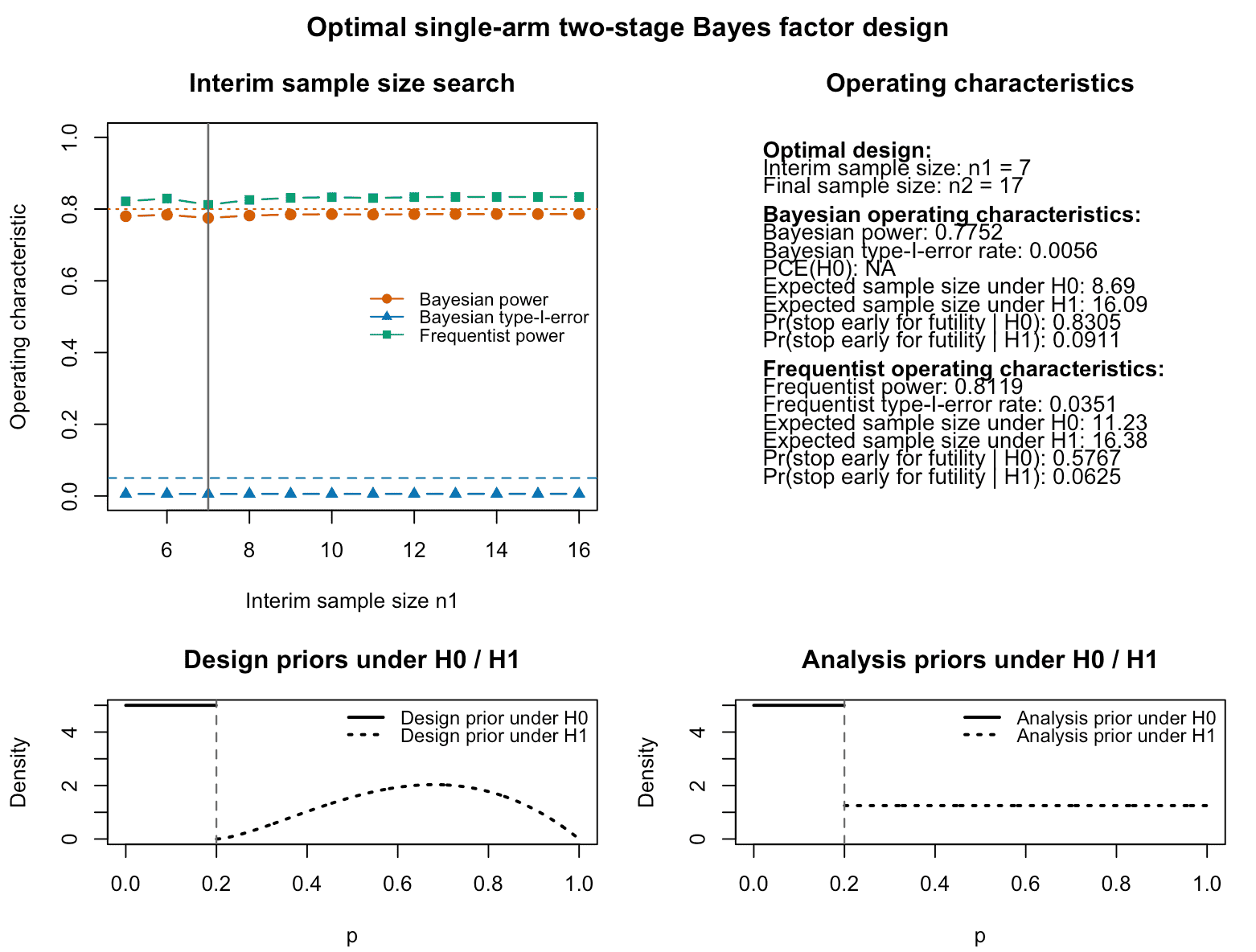

Figure 1: Output of the plot function for an optimal frequentist single-arm two-stage design using Bayes factors. The top left panel shows Bayesian and frequentist power, Bayesian type-I-error for varying interim sample sizes. The top right panel provides information about the optimal frequentist design found by the algorithm and its Bayesian and frequentist operating characteristics. The lower left and right panels visualize the analysis and design priors under the null and alternative hypothesis. For the frequentist operating characteristics, these are irrelevant. They influence only the Bayesian operating characteristics. Under the null hypothesis $H_0:p=p_0$ , the design and analysis priors are point masses at the specified null probability p0.

The plot shows how Bayesian and frequentist operating characteristics vary as a function of the interim sample size, and highlights the optimal choice selected by the algorithm.

Interpreting the frequentist design

Under calibration = "frequentist", the design has the following key properties:

The frequentist type-I error (probability of wrongly rejecting $H_0$ ) is controlled at or below target_freq_type1 when the true response rate is $p = p_0$ .
The frequentist power (probability of rejecting $H_0$ when $p = dp$ ) is at or above target_freq_power.
Among all designs within the specified bounds that satisfy these constraints, the selected design minimizes the expected sample size under $H_0$ . Details are also provided in (Kelter and Pawel 2025b).

The Bayesian operating characteristics are still reported, but they do not drive the calibration; they serve as additional information about how the design performs under the specified design priors.

Practical recommendations for frequentist calibration

When using the frequentist mode in practice:

Choose dp as the clinically relevant response rate under $H_1$ where you want to guarantee power.
Use joint priors under $H_0$ and $H_1$ that reflect realistic beliefs, even though they do not drive the calibration. The resulting Bayesian summaries can be informative.
If no feasible design is found, consider relaxing the targets or enlarging n2_max. In particular, very high power with very small type-I error can be incompatible with tight sample size bounds.

References

Kelter, Riko, and Samuel Pawel. 2025a. Bayesian Power and Sample Size Calculations for Bayes Factors in the Binomial Setting. https://arxiv.org/abs/2502.02914.

Kelter, Riko, and Samuel Pawel. 2025b. The Bayesian Optimal Two-Stage Design for Clinical Phase II Trials Based on Bayes Factors. https://arxiv.org/abs/2511.23144.