Bayesian calibration of two-arm one-stage ROPE designs with binary endpoints

Riko Kelter
Institute of Medical Statistics and Computational Biology
Faculty of Medicine
University of Cologne
Cologne, Germany

15 September 2026

Overview

This vignette illustrates Bayesian predictive and frequentist calibration of a one-stage, equal-allocation, two-arm ROPE equivalence design for a binary endpoint.

The example is motivated by a historical acute maxillary sinusitis setting in which a short-course treatment and a standard active comparator had cure rates near 0.74. The trial results are reported by Luterman et al. (2003). The objective here is methodological: to compare two different ways of calibrating the same posterior ROPE decision rule.

The treatment effect is the risk difference

$$\Delta = p_T - p_C,$$

where $p_C$ and $p_T$ are the control- and treatment-arm response probabilities. Practical equivalence is defined by the ROPE

$$-\delta < \Delta < \delta,$$

with $\delta = 0.10$.

The posterior decision has three outcomes:

• Equivalence: $\Pr(|\Delta| < \delta \mid y_C,y_T) \geq \gamma_{\mathrm{eq}}$.
• Meaningful difference: $\Pr(|\Delta| \geq \delta \mid y_C,y_T) \geq \gamma_{\mathrm{diff}}$.
• Inconclusive: neither condition is met.

We retain weak analysis priors in all examples:

$$p_C \sim \mathrm{Beta}(1,1), \qquad p_T \sim \mathrm{Beta}(1,1).$$

Thus, historical information is used for design-stage predictive averaging, not directly as information in the final posterior analysis.

Load the package

library(bfbin2arm)

Clinical planning distributions

Equivalence design distribution $G_1$

A design prior is needed for Bayesian predictive calibration. It describes plausible future data-generating parameter values when the treatments are expected to be practically equivalent.

For this example, let the baseline response probability follow

$$p_C \sim \mathrm{Beta}(37,13),$$

which has mean $37/(37+13)=0.74$. Let the treatment-control risk difference follow

$$\Delta \sim N(0,0.03^2),$$

truncated to the ROPE $[-0.10,0.10]$, and define

$$p_T=p_C+\Delta.$$

This joint construction concentrates predictive equivalence scenarios near $\Delta=0$, rather than treating all risk differences inside the ROPE as equally plausible.

prior_eq_luterman <- list(
  type = "baseline_difference",

  baseline = list(
    family = "beta",
    shape1 = 37,
    shape2 = 13
  ),

  difference = list(
    family = "normal",
    mean = 0,
    sd = 0.03,
    truncation = c(-0.10, 0.10)
  )
)

Non-equivalence design distribution $G_0$

For the Bayesian predictive false-equivalence probability, use the package’s existing truncated product-Beta non-equivalence design prior:

design_prior_ne_C <- c(37, 13)
design_prior_ne_T <- c(42, 8)

Before truncation, these kernels have means approximately 0.74 and 0.84, respectively. After restriction to $|\Delta|\geq0.10$, this provides a difficult near-boundary non-equivalence scenario.

Two distinct calibrations

The same posterior ROPE decision rule can be calibrated in different ways.

Bayesian predictive calibration

Bayesian predictive operating characteristics average conditional decision probabilities over design distributions:

$$\operatorname{Power}_{G_1}(n) = \Pr_{G_1}(\text{declare equivalence}),$$

and

$$\operatorname{TypeI}_{G_0}(n) = \Pr_{G_0}(\text{declare equivalence}).$$

These are prior-predictive quantities. They answer the question:

Under the specified clinical distributions for equivalence and non-equivalence, how often will this design make each decision?

They do not guarantee pointwise error control at every parameter value outside the ROPE.

Frequentist calibration

Frequentist operating characteristics condition on fixed true response probabilities. For a fixed $(p_C,p_T)$, the equivalence probability is

$$\Pr_{p_C,p_T}(\text{declare equivalence}).$$

In this vignette, frequentist power is evaluated at

$$p_C=p_T=0.74,$$

and frequentist type-I error is approximated by a grid maximum over both ROPE boundaries:

$$p_T=p_C-0.10, \qquad p_T=p_C+0.10,$$

for $p_C\in[0.60,0.85]$.

The frequentist criterion answers a different question:

What is the largest probability of declaring equivalence at the selected fixed boundary scenarios?

Importantly, note that a realistic range of success probabilities $p_C$ for the control arm is selected here. This range $[0.60,0.85]$ is motivated by the historical success rate of about $74\%$. It is of course possible to use even stricter frequentist assumptions by allowing $p_C \in [0.1]$, though this makes little sense in the current trial setting based on the available historical data.

Bayesian predictive calibration

Design specification

The following design uses $\gamma_{\mathrm{eq}}=0.80$ and $\gamma_{\mathrm{diff}}=0.975$. The equivalence threshold was selected as part of predictive calibration so that the Bayesian predictive false-equivalence probability remains at or below 0.05 while obtaining a practically sized trial.

Running this full search can take several minutes, even though it should not take longer than about a minute on a regular desktop computer. With parallel_backend = "psock", candidate sample sizes are evaluated by independent R worker processes. Runtime depends on the number of workers, available physical cores, BLAS threading, and machine load.

design_luterman_bayesian <- design_twoarm_onestage_rope(
  nmin = 80,
  nmax = 240,
  nstep = 1L,

  delta = 0.10,
  gammaeq = 0.80,
  gammadiff = 0.975,

  analysis_prior_C = c(1, 1),
  analysis_prior_T = c(1, 1),

  design_prior_eq = prior_eq_luterman,
  design_prior_ne_C = design_prior_ne_C,
  design_prior_ne_T = design_prior_ne_T,

  calibration = "Bayesian",

  targetpower = 0.80,
  targettype1 = 0.05,

  sustainn = 10L,

  integration = "quantile",
  quad_nodes = 64L,

  parallel = TRUE,
  parallel_backend = "psock",
  ncores = n_workers,

  returngrid = TRUE,
  returnmatrices = TRUE,

  progress = FALSE
)

design_luterman_bayesian

Evaluating 161 candidate per-arm sample sizes using 8 PSOCK worker(s)...

One-stage two-arm ROPE equivalence design
Equal allocation: nC = nT
Search range per arm: 80 to 240 (step 1 )
ROPE half-width delta: 0.1 
Thresholds: gammaeq = 0.8 , gammadiff = 0.975 
Integration: quantile(quantile quadrature; nodes = 64 )
Calibration: Bayesian 
Target predictive power: 0.8 
Target predictive type-I error: 0.05 
Sustain n: 10 

Selected design
nC = 218 , nT = 218 , total N = 436 
Predictive equivalence power: 0.8018 
Predictive false-equivalence probability: 0.0434 
P(meaningful difference | G1): 0.0003 
P(inconclusive | G1): 0.1979 
P(meaningful difference | G0): 0.3828 
P(inconclusive | G0): 0.5738 

Visualize the resulting design

plot(design_luterman_bayesian)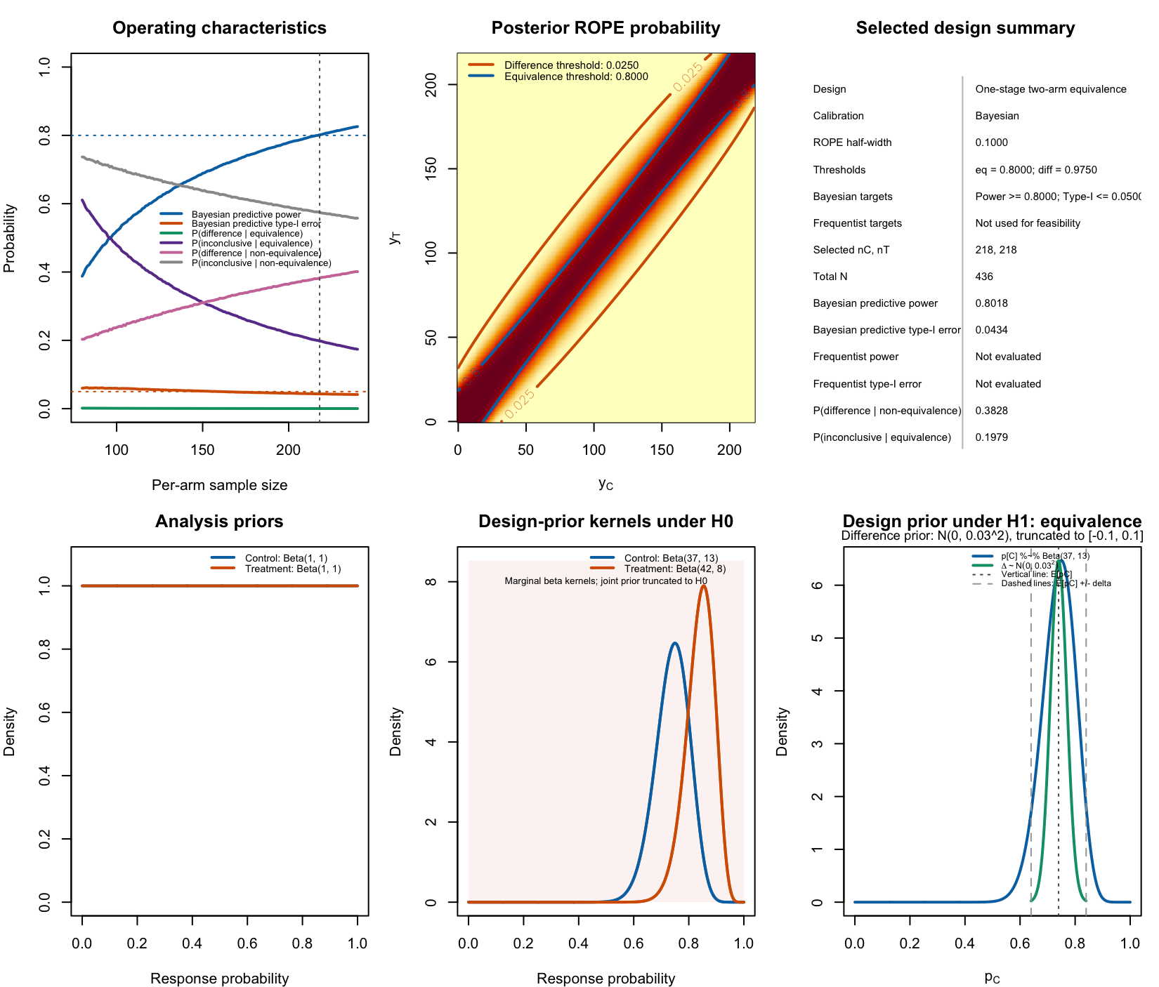

Figure 1: Visualization of the Bayesian calibrated two-arm one-stage ROPE design for a binary endpoint.

The top left panel shows the different operating characteristics for calibration, including the Bayesian power and type-I-error. The middle panel in the top row shows the posterior ROPE probability as a function of the number of successes $y_C$ in the control and $y_T$ in the treatment arm. The top right panel provides a textual summary of the design. The bottom row panels provide an overview about the analysis and design priors.

We can also plot the operating characteristics, the design priors or the heatmap separately:

plot(design_luterman_bayesian, type = "prior")

plot(design_luterman_bayesian, type = "heatmap")

Interpretation

The Bayesian predictive calibration selects an equal-allocation design with

$$n_C=n_T=218, \qquad N=436.$$

Thus, the planned trial randomizes 436 participants in total, with 218 participants assigned to each treatment arm. The final analysis uses weak $\mathrm{Beta}(1,1)$ analysis priors for both response probabilities, so the posterior decision is driven primarily by the trial data rather than by the historical information used to construct the design distributions.

Decision rule at the selected sample size

For the selected design, practical equivalence is declared when the posterior probability that the treatment-control risk difference lies in the ROPE $(-0.10,0.10)$ is at least 0.80:

$$\Pr\left( \left|p_T-p_C\right|<0.10 \mid y_C,y_T \right) \geq 0.80.$$

In clinical terms, the study declares equivalence only when the observed data provide at least 80% posterior probability that the absolute difference in cure probabilities is below 10 percentage points.

A meaningful difference is declared only when the posterior probability of being outside the ROPE is at least 0.975:

$$\Pr\left( \left|p_T-p_C\right|\geq0.10 \mid y_C,y_T \right) \geq0.975.$$

All remaining outcome combinations lead to an inconclusive result. Hence, the design has three possible conclusions: equivalence, meaningful non-equivalence, or inconclusive evidence.

Predictive probability of equivalence

Under the equivalence design distribution $G_1$, the selected design has Bayesian predictive equivalence power

$$\Pr_{G_1}(\text{declare equivalence}) = 0.8018.$$

This means that, before observing the new trial data and under the specified planning distribution for clinically equivalent treatments, the trial has an approximately 80.2% probability of declaring equivalence.

The predictive probability is calculated by averaging over both sources of uncertainty represented in $G_1$:

1. uncertainty in the control-arm cure probability, centred near 0.74; and
2. uncertainty in the treatment-control risk difference, concentrated near zero and restricted to the ROPE.

Therefore, 0.8018 is not the probability of declaring equivalence at one fixed pair $(p_C,p_T)$. Instead, it is the expected probability of an equivalence declaration across the clinically plausible equivalence scenarios encoded by $G_1$.

The design also has

$$\Pr_{G_1}(\text{declare meaningful difference}) = 0.0003,$$

and

$$\Pr_{G_1}(\text{inconclusive}) = 0.1979.$$

The three probabilities approximately sum to one:

$$0.8018 + 0.0003 + 0.1979 = 1.0000.$$

Thus, when the treatments are practically equivalent according to the planning distribution, the design is very unlikely to incorrectly declare a meaningful difference. Its main limitation under $G_1$ is not a false difference conclusion, but an inconclusive result: this occurs in about 19.8% of plausible equivalence scenarios.

Predictive false-equivalence probability

Under the non-equivalence design distribution $G_0$, the selected design has Bayesian predictive false-equivalence probability

$$\Pr_{G_0}(\text{declare equivalence}) = 0.0434.$$

This is below the prespecified target of 0.05. In other words, for the clinically relevant non-equivalence scenarios represented by $G_0$, the prior-predictive probability that the trial nevertheless declares equivalence is approximately 4.3%.

This quantity is a Bayesian predictive type-I-error analogue. It is an average over the non-equivalence design distribution, which in this example is restricted to $\left|p_T-p_C\right|\geq0.10$ and concentrates on difficult near-boundary scenarios. It should therefore be interpreted as protection against false equivalence under the prespecified clinical non-equivalence scenarios, rather than as a maximum error probability at every individual parameter value outside the ROPE.

Under $G_0$, the selected design has

$$\Pr_{G_0}(\text{declare meaningful difference}) = 0.3828,$$

and

$$\Pr_{G_0}(\text{inconclusive}) = 0.5738.$$

Again, these probabilities partition the possible trial decisions:

$$0.0434 + 0.3828 + 0.5738 = 1.0000.$$

Consequently, when the treatments are meaningfully different under the specified $G_0$ scenarios, the design most often returns an inconclusive result rather than a positive difference conclusion. This is a direct consequence of the stringent 0.975 threshold for declaring meaningful difference. The design is therefore deliberately conservative in making a difference claim.

Practical interpretation

The selected $218+218$ design is appropriate if the primary development objective is to support a positive equivalence conclusion when the two treatments are expected to have similar cure probabilities and when the planning distributions $G_1$ and $G_0$ are accepted as clinically reasonable.

In particular, the design implies the following prospective commitments:

• If practical equivalence is true in scenarios represented by $G_1$, there is about an 80% predictive chance that the trial will conclude equivalence.

• If the treatments differ by at least 10 percentage points in scenarios represented by $G_0$, the predictive chance of incorrectly declaring equivalence is about 4%.

• The design has a substantial probability of an inconclusive outcome, especially under $G_0$. This is expected because the rule requires very strong posterior evidence to label a difference as meaningful.

• A declaration of equivalence does not mean that the two cure probabilities are identical. It means that the posterior probability of an absolute risk difference smaller than 10 percentage points is at least 0.80.

• An inconclusive result does not establish non-equivalence. It means that the observed data do not reach either the equivalence threshold or the stringent meaningful-difference threshold.

Scope of the Bayesian guarantee

The calibration is conditional on the ROPE, posterior thresholds, analysis priors, and design distributions used here. In particular, the 0.0434 false-equivalence probability is a prior-weighted predictive average under $G_0$. It does not imply that

$$\Pr_{p_C,p_T}(\text{declare equivalence}) \leq 0.05$$

for every fixed parameter pair satisfying $\left|p_T-p_C\right|\geq0.10$.

That stronger pointwise claim is a frequentist calibration objective and is examined separately below. Accordingly, this Bayesian design is best understood as a design optimized for predictive decision performance under explicit, clinically motivated equivalence and non-equivalence scenarios.

The frequentist calibration below will show, however, that a strict frequentist notion of the type-I-error can become very pricy in terms of the required number of patients.

Frequentist calibration

Why the threshold differs

The Bayesian predictive design above controls a prior-weighted average false-equivalence probability under $G_0$. It does not control the largest fixed-parameter false-equivalence probability along the ROPE boundary.

For the same sample size and $\gamma_{\mathrm{eq}}=0.80$, the frequentist boundary type-I error can be much higher than the Bayesian predictive type-I error. Therefore, a more stringent equivalence threshold is used for frequentist calibration.

Here we use:

$$\gamma_{\mathrm{eq}}=0.95, \qquad \gamma_{\mathrm{diff}}=0.975.$$

The planned pointwise frequentist equivalence scenario is $p_C=p_T=0.74$. The type-I-error boundary grid uses $p_C\in[0.60,0.85]$.

Coarse frequentist-calibration search

We first run a coarse calibration by increasing the sample size by $10$ patients via nstep = 10 as the function parameter. This serves to find a suitable sample size range based on which we can refine the calibration sample size range next:

design_luterman_frequentist_coarse <- design_twoarm_onestage_rope(
  nmin = 100,
  nmax = 500,
  nstep = 10L,

  delta = 0.10,
  gammaeq = 0.975,
  gammadiff = 0.975,

  analysis_prior_C = c(1, 1),
  analysis_prior_T = c(1, 1),

  design_prior_eq = prior_eq_luterman,
  design_prior_ne_C = design_prior_ne_C,
  design_prior_ne_T = design_prior_ne_T,

  calibration = "frequentist",

  freq_pC = 0.74,
  freq_delta = 0,

  targetfreqpower = 0.80,
  targetfreqtype1 = 0.05,

  freq_pC_range = c(0.60, 0.85),
  freq_grid_n = 201L,

  sustainn = 1L,

  integration = "quantile",
  quad_nodes = 64L,

  parallel = TRUE,
  parallel_backend = "psock",
  ncores = n_workers,

  returngrid = TRUE,
  returnmatrices = TRUE,

  progress = FALSE
)

design_luterman_frequentist_coarse

Evaluating 41 candidate per-arm sample sizes using 8 PSOCK worker(s)...
Sample-size search completed in 00:30.

One-stage two-arm ROPE equivalence design
Equal allocation: nC = nT
Search range per arm: 100 to 500 (step 10 )
ROPE half-width delta: 0.1 
Thresholds: gammaeq = 0.975 , gammadiff = 0.975 
Integration: quantile(quantile quadrature; nodes = 64 )
Calibration: frequentist 
Target frequentist power: 0.8 
Target frequentist type-I error: 0.05 
Sustain n: 1 

Selected design
nC = 410 , nT = 410 , total N = 820 
Predictive equivalence power: 0.6645 
Predictive false-equivalence probability: 0.0028 
P(meaningful difference | G1): 0.0001 
P(inconclusive | G1): 0.3354 
P(meaningful difference | G0): 0.5063 
P(inconclusive | G0): 0.4909 
Pointwise frequentist equivalence probability: 0.8128 
Boundary-grid frequentist type-I error: 0.0266 

The results indicate that for $n=410$ in each trial arm, the frequentist constraints on power and type-I-error are satisfied.

Local integer search

After locating the first feasible coarse region, perform an integer search around it. The following bounds are deliberately broad; adjust them using the coarse result if necessary. Importantly, we use nstep = 1 intead of nstep = 10 now, so every sample size between our chosen nmin = 390 and nmax = 420 is analyzed:

design_luterman_frequentist_local <- design_twoarm_onestage_rope(
  nmin = 390,
  nmax = 420,
  nstep = 1L,

  delta = 0.10,
  gammaeq = 0.975,
  gammadiff = 0.975,

  analysis_prior_C = c(1, 1),
  analysis_prior_T = c(1, 1),

  design_prior_eq = prior_eq_luterman,
  design_prior_ne_C = design_prior_ne_C,
  design_prior_ne_T = design_prior_ne_T,

  calibration = "frequentist",

  freq_pC = 0.74,
  freq_delta = 0,

  targetfreqpower = 0.80,
  targetfreqtype1 = 0.05,

  freq_pC_range = c(0.60, 0.85),
  freq_grid_n = 401L,

  sustainn = 5L,

  integration = "quantile",
  quad_nodes = 64L,

  parallel = TRUE,
  parallel_backend = "psock",
  ncores = n_workers,

  returngrid = TRUE,
  returnmatrices = TRUE,

  progress = FALSE
)

design_luterman_frequentist_local

Evaluating 31 candidate per-arm sample sizes using 8 PSOCK worker(s)...
Sample-size search completed in 00:30.

One-stage two-arm ROPE equivalence design
Equal allocation: nC = nT
Search range per arm: 390 to 420 (step 1 )
ROPE half-width delta: 0.1 
Thresholds: gammaeq = 0.975 , gammadiff = 0.975 
Integration: quantile(quantile quadrature; nodes = 64 )
Calibration: frequentist 
Target frequentist power: 0.8 
Target frequentist type-I error: 0.05 
Sustain n: 5 

Selected design
nC = 401 , nT = 401 , total N = 802 
Predictive equivalence power: 0.6541 
Predictive false-equivalence probability: 0.0028 
P(meaningful difference | G1): 0.0001 
P(inconclusive | G1): 0.3458 
P(meaningful difference | G0): 0.5020 
P(inconclusive | G0): 0.4952 
Pointwise frequentist equivalence probability: 0.8005 
Boundary-grid frequentist type-I error: 0.0267 

If no feasible design is found in the local range, enlarge nmax. Do not infer frequentist feasibility from Bayesian predictive feasibility.

We plot the design:

plot(design_luterman_frequentist_local)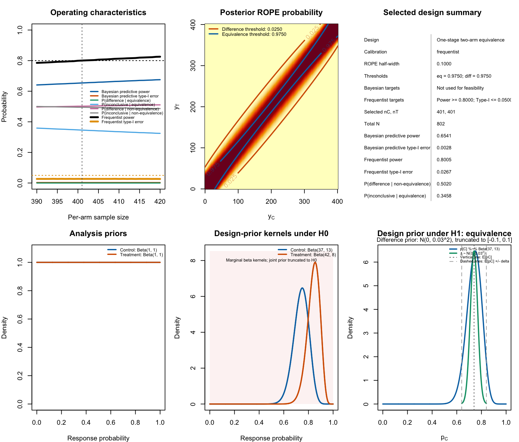

Figure 2: Visualization of the frequentist calibrated two-arm one-stage ROPE design for a binary endpoint.

Interpretation of the frequentist-calibrated design

The local integer search selects an equal-allocation design with

$$n_C=n_T=401, \qquad N=802.$$

Thus, the frequentist-calibrated design requires 401 participants in each treatment arm, for a total of 802 randomized participants. This is substantially larger than the Bayesian predictive design, which selected $218+218=436$ participants. The increase reflects the more demanding frequentist calibration objective: the design must satisfy fixed-parameter operating-characteristic constraints rather than only prior-weighted predictive-average constraints.

The posterior decision rule remains Bayesian. In particular, equivalence is declared when

$$\Pr\left( |p_T-p_C|<0.10 \mid y_C,y_T \right) \geq 0.975.$$

The key difference is therefore not the posterior model used to analyze the trial data, but the criterion used to select the sample size and equivalence threshold during design.

Pointwise frequentist power

The selected design is calibrated at the fixed equivalence scenario

$$p_C=p_T=0.74,$$

for which the true risk difference is

$$\Delta=p_T-p_C=0.$$

At this parameter point, the probability of declaring equivalence is

$$\Pr_{p_C=0.74,p_T=0.74} (\text{declare equivalence}) = 0.8005.$$

Thus, if both treatments truly have a cure probability of 0.74, the planned trial has approximately 80.1% frequentist power to conclude equivalence. This meets the prespecified target of 80%.

This is a conditional, fixed-parameter statement. It does not average over a distribution of plausible response probabilities or treatment effects. The result answers the specific question:

If the true cure probabilities are both 0.74, how often would repeated trials of this design declare equivalence?

The answer is approximately 80 times in 100 repeated trials.

Boundary-grid false-equivalence probability

The frequentist type-I-error calculation evaluates scenarios on both boundaries of the ROPE:

$$p_T=p_C-0.10,$$

and

$$p_T=p_C+0.10,$$

over the clinically motivated control-rate range

$$p_C\in[0.60,0.85].$$

These are the parameter configurations at which the true risk difference is exactly at the practical-equivalence boundary:

$$|p_T-p_C|=0.10.$$

At these boundary scenarios, declaring equivalence is a false-equivalence decision under the frequentist null hypothesis. The selected design has maximum boundary-grid false-equivalence probability

$$\max_{p_C\in[0.60,0.85]} \Pr_{p_C,p_T} (\text{declare equivalence}) = 0.0267.$$

This is below the prespecified target of 0.05. Therefore, within the evaluated grid of boundary scenarios, the probability of incorrectly declaring equivalence is at most approximately 2.7%.

The reported value is conservative relative to the target: it is materially smaller than 0.05 because the sample size is determined jointly by the power requirement, integer sample-size constraints, and the requirement that five consecutive candidate sample sizes satisfy the feasibility criteria (sustainn = 5L).

Meaning of sustainn = 5

The local search uses

sustainn = 5L

rather than accepting the first single feasible candidate sample size. A sample size is selected only when it is the first member of a run of five consecutive evaluated sample sizes that all meet the frequentist feasibility criteria.

This requirement reduces the chance that a design is selected solely because of an isolated numerical irregularity or a local non-monotonicity in the computed operating characteristics. Consequently, the chosen design should be interpreted as a stable feasible region in the local integer search, not merely as the first individual value that happens to cross the target.

Relation to the Bayesian operating characteristics

Although the sample size was selected using frequentist constraints, the function also reports Bayesian predictive operating characteristics for the same posterior decision rule. At $n_C=n_T=401$, these are

$$\Pr_{G_1}(\text{declare equivalence})=0.6541,$$

and

$$\Pr_{G_0}(\text{declare equivalence})=0.0028.$$

The predictive equivalence probability of 0.6541 is lower than the 0.80 frequentist target because the two quantities address different design questions.

The frequentist power calculation fixes the true scenario at

$$p_C=p_T=0.74.$$

In contrast, the Bayesian predictive calculation averages across the full equivalence design distribution $G_1$, including values of $p_C$ and $p_T-p_C$ throughout the ROPE. Some of these values lie close to the ROPE boundaries, where an equivalence declaration is more difficult. Therefore, a frequentist power of approximately 80% at $\Delta=0$ need not imply a Bayesian predictive equivalence probability of 80%.

Similarly, the Bayesian predictive false-equivalence probability of 0.0028 is an average over the specified non-equivalence distribution $G_0$, whereas the frequentist result of 0.0267 is a maximum over the selected fixed boundary grid. The maximum is expected to be larger than a prior-weighted average when the design distribution gives appreciable weight to non-boundary scenarios.

Practical implications

The frequentist-calibrated design provides the following operating commitments under the specified design assumptions:

• If the true cure probabilities are $p_C=p_T=0.74$, the probability of declaring equivalence is approximately 80.1%.

• If the true treatment-control difference lies on either ROPE boundary, $|p_T-p_C|=0.10$, and the control cure probability lies in $[0.60,0.85]$, the estimated probability of falsely declaring equivalence is no larger than approximately 2.7% on the evaluated grid.

• The equivalence conclusion requires stronger posterior evidence than in the Bayesian predictive design because $\gamma_{\mathrm{eq}}=0.975$, rather than $\gamma_{\mathrm{eq}}=0.80$.

• The stricter threshold and conditional error-control objective increase the required total sample size from 436 to 802 participants.

• A conclusion of equivalence still does not mean that the treatment effects are exactly identical. It means that the observed data provide at least 97.5% posterior probability that the absolute difference in cure probabilities is less than 10 percentage points.

Scope of the frequentist guarantee

The reported false-equivalence probability is a numerical maximum over the specified finite boundary grid:

$$p_C\in[0.60,0.85], \qquad p_T=p_C\pm0.10.$$

It is therefore an approximation to worst-case boundary error control over that clinically chosen range, rather than a formal proof of a global supremum over every possible response probability in $[0,1]$.

The validity and relevance of this calibration depend on prespecifying:

• the ROPE half-width $\delta=0.10$;
• the equivalence threshold $\gamma_{\mathrm{eq}}=0.975$;
• the fixed power scenario $p_C=p_T=0.74$;
• the control-rate range $[0.60,0.85]$;
• the boundary-grid density (freq_grid_n = 401L); and
• the target frequentist power and type-I-error levels.

Accordingly, this design is appropriate when the principal objective is frequentist protection against false equivalence at clinically credible ROPE boundary scenarios, while retaining a Bayesian posterior-probability decision rule for the final analysis.

Bayesian calibration with a PCE(H0) requirement

The initial Bayesian-predictive design was calibrated to achieve a high probability of declaring practical equivalence under $G_1$, while limiting the predictive probability of falsely declaring equivalence under $G_0$. This is appropriate when the principal objective is an equivalence claim.

However, a design can satisfy those two requirements while still having a substantial probability of an inconclusive outcome when meaningful non-equivalence is true. In the original Bayesian design with $n_C=n_T=218$, the predictive probability of declaring meaningful non-equivalence under $G_0$ was only

$$\Pr_{G_0}(\text{declare meaningful non-equivalence})=0.3828.$$

Thus, under the non-equivalence planning distribution, the original design had only about a 38% probability of obtaining compelling evidence that the treatments differ by at least the ROPE half-width. Most of the remaining probability corresponded to an inconclusive result rather than to a false equivalence conclusion.

The targetpce_h0 argument allows this operating characteristic to become an explicit Bayesian calibration criterion. Under the notation used here,

$$H_0:\ |p_T-p_C|\geq\delta$$

denotes meaningful non-equivalence, whereas

$$H_1:\ |p_T-p_C|<\delta$$

denotes practical equivalence. The probability of compelling evidence for $H_0$ is therefore

$$\operatorname{PCE}_{H_0}(n) = \Pr_{G_0} \left[ \Pr\left( |p_T-p_C|\geq\delta \mid y_C,y_T \right) \geq\gamma_{\mathrm{diff}} \right].$$

Equivalently, PCE(H0) is the Bayesian predictive probability of declaring a meaningful difference when the non-equivalence design distribution $G_0$ holds.

In the following calibration, we retain the original Bayesian requirements

$$\operatorname{PCE}_{H_1}(n) = \Pr_{G_1}(\text{declare equivalence}) \geq0.80,$$

and

$$\Pr_{G_0}(\text{declare equivalence}) \leq0.05,$$

but additionally require

$$\operatorname{PCE}_{H_0}(n)\geq0.50.$$

The resulting design is therefore required to have at least a 50% prior-predictive probability of reaching a compelling correct non-equivalence conclusion under $G_0$.

design_luterman_bayesian_pce_h0 <- design_twoarm_onestage_rope(
  nmin = 80L,
  nmax = 450L,
  nstep = 1L,

  delta = 0.10,
  gammaeq = 0.80,
  gammadiff = 0.975,

  analysis_prior_C = c(1, 1),
  analysis_prior_T = c(1, 1),

  design_prior_eq = prior_eq_luterman,
  design_prior_ne_C = design_prior_ne_C,
  design_prior_ne_T = design_prior_ne_T,

  calibration = "Bayesian",

  targetpower = 0.80,
  targettype1 = 0.05,
  targetpce_h0 = 0.50,

  sustainn = 10L,

  integration = "quantile",
  quad_nodes = 64L,

  parallel = TRUE,
  parallel_backend = "psock",
  ncores = n_workers,

  returngrid = TRUE,
  returnmatrices = TRUE,

  progress = FALSE
)

design_luterman_bayesian_pce_h0

Evaluating 371 candidate per-arm sample sizes using 11 PSOCK worker(s)...
Sample-size search completed in 05:44.

One-stage two-arm ROPE equivalence design
Equal allocation: nC = nT
Search range per arm: 80 to 450 (step 1 )
ROPE half-width delta: 0.1 
Thresholds: gammaeq = 0.8 , gammadiff = 0.975 
Integration: quantile(quantile quadrature; nodes = 64 )
Calibration: Bayesian 
Target PCE(H1): 0.8000 
Maximum predictive false-equivalence probability: 0.0500 
Target PCE(H0): 0.5000 
Sustain n: 10 

Selected design
nC = 397 , nT = 397 , total N = 794 
PCE(H1), practical equivalence: 0.9174 
Predictive false-equivalence probability: 0.0325 
P(meaningful difference | G1): 0.0001 
P(inconclusive | G1): 0.0825 
PCE(H0), meaningful non-equivalence: 0.5004 
P(inconclusive | G0): 0.4671 
PCE(H0) target satisfied: TRUE 

Interpretation

Adding a minimum probability of compelling evidence for $H_0$ changes the purpose of the Bayesian calibration. The design is no longer required only to support an equivalence conclusion when practical equivalence holds and to avoid false equivalence when meaningful non-equivalence holds. It is also required to have a substantial probability of reaching a compelling correct non-equivalence conclusion when $H_0$ holds.

In this vignette, the hypotheses are defined as

$$H_0:\ |p_T-p_C|\geq0.10,$$

which represents meaningful non-equivalence, and

$$H_1:\ |p_T-p_C|<0.10,$$

which represents practical equivalence.

The additional criterion is the predictive probability of compelling evidence for $H_0$:

$$\operatorname{PCE}_{H_0}(n) = \Pr_{G_0} \left[ \Pr\left( |p_T-p_C|\geq0.10 \mid y_C,y_T \right) \geq0.975 \right].$$

Equivalently, $\operatorname{PCE}_{H_0}$ is the Bayesian predictive probability of declaring meaningful non-equivalence when the non-equivalence design distribution $G_0$ applies.

The new calibration requires

$$\operatorname{PCE}_{H_1}(n) = \Pr_{G_1}(\text{declare equivalence}) \geq0.80,$$

$$\Pr_{G_0}(\text{declare equivalence}) \leq0.05,$$

and additionally

$$\operatorname{PCE}_{H_0}(n)\geq0.50.$$

The selected design has

$$n_C=n_T=397, \qquad N=794.$$

Thus, 397 participants are allocated to each arm, for a total sample size of 794 participants.

Under the equivalence design distribution $G_1$, the selected design has

$$\operatorname{PCE}_{H_1} = \Pr_{G_1}(\text{declare equivalence}) = 0.9174.$$

Therefore, when practical equivalence holds according to the clinically specified equivalence planning distribution, the trial has approximately a 91.7% predictive probability of declaring equivalence. This exceeds the required minimum predictive equivalence probability of 80%.

The selected design also has a very small predictive probability of incorrectly declaring meaningful non-equivalence under $G_1$:

$$\Pr_{G_1}(\text{declare meaningful non-equivalence}) = 0.0001.$$

The remaining probability under $G_1$ corresponds to an inconclusive trial result:

$$\Pr_{G_1}(\text{inconclusive})=0.0825.$$

Hence, under the equivalence planning distribution, the design is expected to declare equivalence in most trials, is extremely unlikely to make a compelling but incorrect non-equivalence conclusion, and produces an inconclusive result in approximately 8.3% of trials.

Under the non-equivalence design distribution $G_0$, the predictive probability of falsely declaring equivalence is

$$\Pr_{G_0}(\text{declare equivalence})=0.0325.$$

This remains below the prespecified maximum of 0.05. Thus, even after adding the PCE(H0) requirement, the design retains the desired predictive protection against a false equivalence conclusion.

Most importantly, the selected design achieves

$$\operatorname{PCE}_{H_0} = \Pr_{G_0}(\text{declare meaningful non-equivalence}) = 0.5004.$$

Therefore, when meaningful non-equivalence scenarios represented by $G_0$ hold, the trial has approximately a 50.0% predictive probability of producing compelling posterior evidence for $H_0$. This satisfies the target

$$\operatorname{PCE}_{H_0}\geq0.50.$$

The remaining predictive probability under $G_0$ is primarily attributable to an inconclusive result:

$$\Pr_{G_0}(\text{inconclusive})=0.4671.$$

The predictive decision probabilities under $G_0$ therefore partition as

$$\Pr_{G_0}(\text{false equivalence}) + \Pr_{G_0}(\text{compelling evidence for }H_0) + \Pr_{G_0}(\text{inconclusive}) = 1,$$

or numerically,

$$0.0325+0.5004+0.4671=1.0000.$$

The additional PCE(H0) criterion has an important practical consequence. A design can obtain a low false-equivalence probability partly by returning many inconclusive results whenever meaningful non-equivalence is true. Such a design is conservative about declaring equivalence, but it may not be very informative in the opposite direction.

Requiring

$$\operatorname{PCE}_{H_0}\geq0.50$$

prevents the design from meeting the false-equivalence target merely by being inconclusive. It requires the trial to have a meaningful chance of delivering a decisive and correct non-equivalence conclusion when the treatments differ by at least the clinically relevant margin.

This additional decisiveness increases the required sample size. The original Bayesian-predictive calibration selected

$$n_C=n_T=218, \qquad N=436,$$

and had

$$\operatorname{PCE}_{H_0}=0.3828.$$

It therefore controlled predictive false equivalence but did not meet a minimum PCE(H0) target of 0.50. Adding the PCE(H0) requirement increases the selected design to

$$n_C=n_T=397, \qquad N=794.$$

The larger sample size reflects the fact that the design must now be informative in both directions:

• It should provide compelling evidence for practical equivalence when $H_1$ holds.

• It should avoid falsely declaring equivalence when $H_0$ holds.

• It should also provide compelling evidence for meaningful non-equivalence with at least 50% predictive probability when $H_0$ holds.

The PCE(H0)-constrained Bayesian design remains distinct from the frequentist calibration. Its guarantees are predictive averages over the clinically specified design distributions $G_1$ and $G_0$. In particular, it does not guarantee that the conditional probability of falsely declaring equivalence is below 0.05 at every fixed parameter point on the ROPE boundary.

Nevertheless, this criterion is a useful strength of the Bayesian design framework. It allows trial planning to directly target the probability of a scientifically compelling conclusion under both practical equivalence and meaningful non-equivalence, rather than treating a large probability of inconclusive trials as acceptable by default.

AURIEL-PsO: a smaller binary-endpoint equivalence example

The AURIEL-PsO study was a randomized, double-blind phase-III equivalence trial comparing the adalimumab biosimilar MSB11022 with reference adalimumab in patients with moderate-to-severe chronic plaque psoriasis. The primary efficacy endpoint was a binary response indicator: achievement of at least 75% improvement in the Psoriasis Area and Severity Index at week 16 (PASI 75).

The per-protocol analysis included 203 participants in the MSB11022 group and 191 participants in the reference-adalimumab group. PASI-75 response was observed in 182/203 participants (89.7%) receiving MSB11022 and 175/191 participants (91.6%) receiving reference adalimumab. The observed response difference was therefore

$$\widehat{\Delta} = \widehat{p}_{T}-\widehat{p}_{C} = \frac{182}{203}-\frac{175}{191} = -0.019,$$

where treatment is MSB11022 and control is reference adalimumab.

The original equivalence analysis used an absolute response-rate equivalence margin of $\pm0.18$. The resulting 90% confidence interval for the treatment-control difference, $(-0.0683,0.0306)$, was contained in that margin. Therefore, the original study concluded that no meaningful efficacy difference was demonstrated on the PASI-75 endpoint (Hercogová et al. 2020).

For the ROPE-based design illustration, we use the same clinically motivated absolute margin:

$$H_0:\ |p_T-p_C|\geq0.18, \qquad H_1:\ |p_T-p_C|<0.18.$$

Thus, $H_0$ represents meaningful non-equivalence and $H_1$ represents practical equivalence. This is a natural fit for the two-arm beta-binomial ROPE model because the endpoint is binary and the equivalence estimand is an absolute risk difference.

Historical response data

n_msb11022 <- 203L
y_msb11022 <- 182L

n_adalimumab <- 191L
y_adalimumab <- 175L

p_msb11022 <- y_msb11022 / n_msb11022
p_adalimumab <- y_adalimumab / n_adalimumab

observed_difference <- p_msb11022 - p_adalimumab

data.frame(
  treatment = c(
    "MSB11022",
    "Reference adalimumab"
  ),
  responders = c(
    y_msb11022,
    y_adalimumab
  ),
  nonresponders = c(
    n_msb11022 - y_msb11022,
    n_adalimumab - y_adalimumab
  ),
  total = c(
    n_msb11022,
    n_adalimumab
  ),
  response_probability = c(
    p_msb11022,
    p_adalimumab
  )
)
#>              treatment responders nonresponders total response_probability
#> 1             MSB11022        182            21   203            0.8965517
#> 2 Reference adalimumab        175            16   191            0.9162304

observed_difference
#> [1] -0.01967864

The observed PASI-75 response probabilities are approximately

$$\widehat{p}_{T}=0.897, \qquad \widehat{p}_{C}=0.916,$$

with an observed treatment-control difference of approximately $-0.019$. The historical results are used here to motivate planning distributions. They are not used as analysis priors: the final trial analysis retains weak $\mathrm{Beta}(1,1)$ priors in both arms.

Planning distributions

The PASI-75 response rate for reference adalimumab was approximately 0.916 in the per-protocol analysis. For the equivalence design distribution $G_1$, we centre the control response probability near 0.90 and centre the treatment-control risk difference at zero.

The beta distribution

$$p_C\sim\operatorname{Beta}(46,5)$$

has mean

$$\frac{46}{46+5}=0.902.$$

Its effective sample size of 51 is deliberately smaller than the historical per-protocol reference-arm sample size. This discounts historical information when constructing a prospective planning distribution.

For the treatment-control difference under practical equivalence, we use

$$\Delta=p_T-p_C \sim N(0,0.06^2),$$

truncated to the ROPE $[-0.18,0.18]$. This places most planning weight near no response-rate difference while allowing clinically small deviations within the prespecified equivalence margin.

prior_eq_auriel <- list(
  type = "baseline_difference",

  baseline = list(
    family = "beta",
    shape1 = 46,
    shape2 = 5
  ),

  difference = list(
    family = "normal",
    mean = 0,
    sd = 0.06,
    truncation = c(-0.18, 0.18)
  )
)

For the non-equivalence distribution $G_0$, we use an illustrative near-boundary scenario in which the reference-adalimumab response probability remains high but the MSB11022 response probability is meaningfully lower.

design_prior_ne_C_auriel <- c(46, 5)
design_prior_ne_T_auriel <- c(36, 14)

Before truncation, these beta kernels have means

$$E(p_C)=\frac{46}{51}=0.902, \qquad E(p_T)=\frac{36}{50}=0.720.$$

Hence, before the explicit non-equivalence restriction, the treatment-control difference is centred approximately at

$$0.720-0.902=-0.182.$$

Restricting the product-Beta distribution to

$$|p_T-p_C|\geq0.18$$

therefore creates a difficult non-equivalence planning distribution close to the lower ROPE boundary. This choice should be regarded as an illustrative planning scenario and should be varied in sensitivity analyses.

Bayesian predictive calibration

The following calculation uses the posterior thresholds

$$\gamma_{\mathrm{eq}}=0.80, \qquad \gamma_{\mathrm{diff}}=0.975.$$

The design is required to have at least 80% predictive probability of declaring practical equivalence under $G_1$ and no more than 5% predictive probability of falsely declaring equivalence under $G_0$.

design_auriel_bayesian <- design_twoarm_onestage_rope(
  nmin = 20L,
  nmax = 350L,
  nstep = 1L,

  delta = 0.18,
  gammaeq = 0.80,
  gammadiff = 0.975,

  analysis_prior_C = c(1, 1),
  analysis_prior_T = c(1, 1),

  design_prior_eq = prior_eq_auriel,
  design_prior_ne_C = design_prior_ne_C_auriel,
  design_prior_ne_T = design_prior_ne_T_auriel,

  calibration = "Bayesian",

  targetpower = 0.80,
  targettype1 = 0.05,

  sustainn = 10L,

  integration = "quantile",
  quad_nodes = 64L,

  parallel = TRUE,
  parallel_backend = "psock",
  ncores = n_workers,

  returngrid = TRUE,
  returnmatrices = TRUE,

  progress = FALSE
)

design_auriel_bayesian

One-stage two-arm ROPE equivalence design
Equal allocation: nC = nT
Search range per arm: 20 to 250 (step 1 )
ROPE half-width delta: 0.18 
Thresholds: gammaeq = 0.8 , gammadiff = 0.975 
Integration: quantile(quantile quadrature; nodes = 64 )
Calibration: Bayesian 
Target PCE(H1): 0.8000 
Maximum predictive false-equivalence probability: 0.0500 
Sustain n: 10 

Selected design
nC = 172 , nT = 172 , total N = 344 
PCE(H1), practical equivalence: 0.9798 
Predictive false-equivalence probability: 0.0494 
P(meaningful difference | G1): 0.0001 
P(inconclusive | G1): 0.0201 
PCE(H0), meaningful non-equivalence: 0.3355 
P(inconclusive | G0): 0.6151 

The search range begins at 20 participants per arm because the ROPE is wider than in the sinusitis example and the PASI-75 response probability is high. The upper bound of 350 participants per arm is nearly exhausted here, as 344 patients are required. If no feasible design is found, increase nmax; if the selected design occurs well inside the range, rerun a narrower local search to verify the result.

plot(design_auriel_bayesian)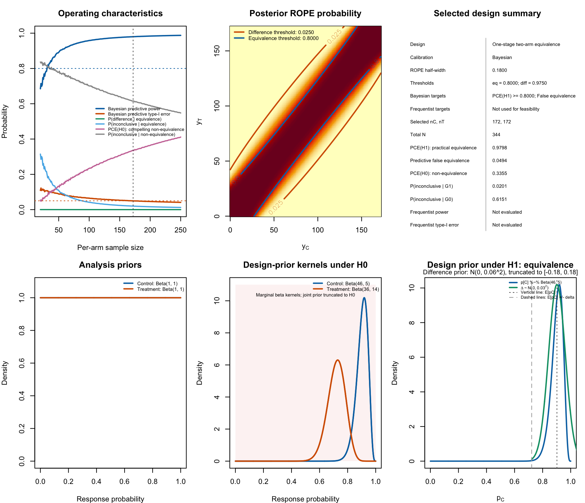

Figure 4: Visualization of the two-arm single-stage ROPE design’s operating characteristics for the AURIEL trial example.

Bayesian calibration with PCE(H0)

The ordinary Bayesian calibration controls the predictive probability of a false equivalence declaration under $G_0$. It does not, by itself, require a high probability of reaching a compelling correct non-equivalence conclusion when $H_0$ holds.

To require informative decisions in both directions, add the criterion

$$\operatorname{PCE}_{H_0} = \Pr_{G_0}(\text{declare meaningful non-equivalence}) \geq0.50.$$

Also, we use a more informative non-equivalence prior here. This is relevant insofar as the earlier prior under non-equivalence was very close to the ROPE boundary. This makes it difficult for the ROPE to express meaningful non-equivalence under that prior. Thus, centering the prior at clearer non-equivalence scenarios allows to obtain a smaller trial sample size, even when adding the constraint on meaningful non-equivalence.

design_prior_ne_C_auriel <- c(
  46,
  5
)

design_prior_ne_T_auriel_clear <- c(
  33,
  18
)

design_auriel_bayesian_pce_h0_clear <- design_twoarm_onestage_rope(
  nmin = 20L,
  nmax = 300L,
  nstep = 1L,

  delta = 0.18,
  gammaeq = 0.80,
  gammadiff = 0.975,

  analysis_prior_C = c(1, 1),
  analysis_prior_T = c(1, 1),

  design_prior_eq = prior_eq_auriel,

  design_prior_ne_C = design_prior_ne_C_auriel,
  design_prior_ne_T = design_prior_ne_T_auriel_clear,

  calibration = "Bayesian",

  targetpower = 0.80,
  targettype1 = 0.05,
  targetpce_h0 = 0.50,

  sustainn = 10L,

  integration = "quantile",
  quad_nodes = 64L,

  parallel = TRUE,
  parallel_backend = "psock",
  ncores = n_workers,

  returngrid = TRUE,
  returnmatrices = TRUE,

  progress = FALSE
)

design_auriel_bayesian_pce_h0_clear

One-stage two-arm ROPE equivalence design
Equal allocation: nC = nT
Search range per arm: 20 to 300 (step 1 )
ROPE half-width delta: 0.18 
Thresholds: gammaeq = 0.8 , gammadiff = 0.975 
Integration: quantile(quantile quadrature; nodes = 64 )
Calibration: Bayesian 
Target PCE(H1): 0.8000 
Maximum predictive false-equivalence probability: 0.0500 
Target PCE(H0): 0.5000 
Sustain n: 10 

Selected design
nC = 146 , nT = 146 , total N = 292 
PCE(H1), practical equivalence: 0.9749 
Predictive false-equivalence probability: 0.0268 
P(meaningful difference | G1): 0.0001 
P(inconclusive | G1): 0.0251 
PCE(H0), meaningful non-equivalence: 0.5016 
P(inconclusive | G0): 0.4716 
PCE(H0) target satisfied: TRUE 

Thus, $146$ patients per trial arm suffice. Note that the PCE(H0)-constrained calibration asks the design to satisfy all three predictive requirements:

$$\Pr_{G_1}(\text{declare equivalence})\geq0.80,$$

$$\Pr_{G_0}(\text{declare equivalence})\leq0.05,$$

and

$$\Pr_{G_0}(\text{declare meaningful non-equivalence})\geq0.50.$$

The third requirement prevents a design from controlling false equivalence mainly by producing inconclusive outcomes under $G_0$.

Sensitivity of PCE(H0) to the non-equivalence design distribution

The preceding ordinary Bayesian calibration selected a design with

$$n_C=n_T=172, \qquad N=344,$$

using the near-boundary non-equivalence design distribution. This design was calibrated to achieve high predictive probability of declaring practical equivalence under $G_1$ and to control the predictive probability of falsely declaring equivalence under $G_0$. It did not impose a minimum probability of compelling evidence for meaningful non-equivalence.

For that design, the predictive probability of compelling evidence for $H_0$ was

$$\operatorname{PCE}_{H_0} = \Pr_{G_0}(\text{declare meaningful non-equivalence}) = 0.3355.$$

Thus, although the ordinary Bayesian design controls predictive false equivalence at the prespecified 5% level, it has only about a 33.6% predictive probability of declaring meaningful non-equivalence under the near-boundary $G_0$ distribution. Most remaining $G_0$ scenarios produce an inconclusive result.

The targetpce_h0 argument allows the probability of compelling evidence for $H_0$ to become an explicit calibration requirement. This extension is particularly informative because it reveals how the required sample size depends on the clinical non-equivalence scenarios encoded by $G_0$.

In both sensitivity analyses below, the ROPE and posterior decision thresholds are held fixed:

$$H_0:\ |p_T-p_C|\geq0.18, \qquad H_1:\ |p_T-p_C|<0.18,$$

$$\gamma_{\mathrm{eq}}=0.80, \qquad \gamma_{\mathrm{diff}}=0.975.$$

The PCE(H0)-constrained calibration requires all of the following:

$$\Pr_{G_1}(\text{declare equivalence})\geq0.80,$$

$$\Pr_{G_0}(\text{declare equivalence})\leq0.05,$$

and

$$\operatorname{PCE}_{H_0} = \Pr_{G_0}(\text{declare meaningful non-equivalence}) \geq0.50.$$

The two sensitivity analyses differ only in the non-equivalence planning distribution $G_0$.

Near-boundary non-equivalence

The first non-equivalence design distribution is centred close to the lower ROPE boundary. Its marginal means are approximately

$$E_{G_0}(p_C) = \frac{46}{46+5} = 0.902,$$

and

$$E_{G_0}(p_T) = \frac{36}{36+14} = 0.720.$$

The corresponding approximate treatment-control difference is

$$E_{G_0}(p_T-p_C) \approx 0.720-0.902 = -0.182.$$

This is only slightly outside the lower ROPE boundary:

$$-\delta=-0.18.$$

Under this near-boundary $G_0$ specification, no sustained feasible design was found in the search range from 20 to 300 participants per arm when requiring

$$\operatorname{PCE}_{H_0}\geq0.50.$$

The limiting criterion was PCE(H0), rather than PCE(H1) or predictive false-equivalence control. The first sample sizes satisfying each individual criterion were:

Criterion	Requirement	First qualifying per-arm sample size
PCE(H1): declare practical equivalence under $G_1$	$\geq0.80$	31
Predictive false equivalence under $G_0$	$\leq0.05$	169
PCE(H0): declare meaningful non-equivalence under $G_0$	$\geq0.50$	Not reached by $n=300$

At sample size $300$,

$$n_C=n_T=300, \qquad N=600,$$

the predictive operating characteristics were

$$\operatorname{PCE}_{H_1}=0.9900,$$

$$\Pr_{G_0}(\text{declare equivalence})=0.0376,$$

and

$$\operatorname{PCE}_{H_0}=0.4472.$$

Therefore, the near-boundary design meets the PCE(H1) and predictive false-equivalence requirements but does not achieve the desired 50% probability of compelling evidence for $H_0$. Only for $N=344$ does the design meet the target constraints on the probability of compelling evidence for $H_0$.

This is scientifically expected. A difference that lies only marginally outside the ROPE is difficult to distinguish from practical equivalence. Because the meaningful-non-equivalence decision requires posterior probability at least 0.975 outside the ROPE, a substantial proportion of repeated trials remain inconclusive under such near-boundary scenarios.

Clearly non-equivalent planning distribution

The second analysis retains the same ROPE, posterior thresholds, equivalence design distribution $G_1$, and PCE(H0) target. It changes only the non-equivalence design distribution to represent a more clearly clinically important loss of efficacy.

The control response probability remains centred near 0.90:

$$E_{G_0}(p_C) = \frac{46}{46+5} = 0.902.$$

The MSB11022 response probability is now centred near 0.65:

$$E_{G_0}(p_T) = \frac{33}{33+18} = 0.647.$$

The approximate treatment-control difference is consequently

$$E_{G_0}(p_T-p_C) \approx 0.647-0.902 = -0.255.$$

This difference is clearly outside the lower ROPE boundary of $-0.18$. It represents an anticipated PASI-75 response-rate loss of about 25 percentage points relative to reference adalimumab, rather than a difference that is only just beyond the clinically acceptable margin.

Under this $G_0$ specification, the PCE(H0)-constrained Bayesian calibration selects

$$n_C=n_T=146, \qquad N=292.$$

The selected design satisfies all three predictive calibration requirements:

Operating characteristic	Value	Requirement
PCE(H1): declare practical equivalence under $G_1$	0.9749	$\geq0.80$
Predictive false-equivalence probability under $G_0$	0.0268	$\leq0.05$
PCE(H0): declare meaningful non-equivalence under $G_0$	0.5016	$\geq0.50$

The remaining predictive decision probabilities are

$$\Pr_{G_1}(\text{declare meaningful non-equivalence})=0.0001,$$

$$\Pr_{G_1}(\text{inconclusive})=0.0251,$$

and

$$\Pr_{G_0}(\text{inconclusive})=0.4716.$$

The selected sample size is primarily determined by the PCE(H0) requirement: the chosen design is the first sustained feasible sample-size region for which the probability of compelling evidence for $H_0$ reaches the prespecified 50% target.

Implications for Bayesian design priors

These results show that the non-equivalence design distribution $G_0$ is a substantive clinical input, not merely a technical component of the calculation. It specifies the non-equivalence scenarios in which the trial is expected to provide compelling evidence that the treatments differ by at least the clinically meaningful margin.

The near-boundary specification asks:

Can the trial reliably distinguish practical equivalence from a treatment difference that is only marginally larger than the accepted clinical equivalence margin?

The clearly non-equivalent specification asks:

Can the trial reliably identify an efficacy difference that is clearly beyond the accepted clinical equivalence margin?

Both questions are scientifically relevant, but they lead to markedly different sample-size requirements. A high target PCE(H0) is costly when $G_0$ concentrates close to the ROPE boundary because many trials will reasonably remain inconclusive. In contrast, a $G_0$ distribution centered further from the boundary corresponds to a more distinguishable clinically meaningful difference and can yield a substantially smaller calibrated design.

The selected $146+146$ design has total sample size

$$N=292,$$

which is smaller than the 394 participants in the AURIEL-PsO per-protocol analysis. This comparison should not be interpreted as showing that 292 participants would reproduce or replace the original trial’s frequentist equivalence calculation. Rather, $N=292$ is the sample size selected by the present Bayesian ROPE decision rule under the explicitly stated planning distributions, posterior thresholds, and predictive calibration targets.

The sensitivity analysis illustrates a central advantage of the Bayesian design framework: it allows the trial to be calibrated not only to limit a wrong equivalence conclusion, but also to target a clinically meaningful probability of compelling correct evidence for non-equivalence. The price of that additional decisiveness depends directly on the non-equivalence scenarios that investigators regard as clinically plausible.

Calibration modes

The function supports four modes. They differ only in which constraints determine feasibility; the posterior decision rule is unchanged for a fixed $\delta$, $\gamma_{\mathrm{eq}}$, $\gamma_{\mathrm{diff}}$, and analysis priors.

Mode	Required criteria
"Bayesian"	power >= targetpower and type1 <= targettype1
"frequentist"	freqpower >= targetfreqpower and freqtype1 <= targetfreqtype1
"hybrid"	power >= targetpower and freqtype1 <= targetfreqtype1
"full"	All Bayesian and frequentist criteria

In the present example:

• The Bayesian mode with $\gamma_{\mathrm{eq}}=0.80$ prioritizes predictive decision performance under the prespecified $G_1$ and $G_0$ distributions.
• The frequentist mode with $\gamma_{\mathrm{eq}}=0.975$ prioritizes pointwise power and approximate worst-case boundary error control.
• The hybrid mode would require predictive Bayesian power and frequentist boundary type-I-error control.
• The full mode would require all four targets simultaneously and is expected to be the most demanding.

Boundary-error visualization

A useful additional diagnostic plots the fixed-parameter probability of declaring equivalence on the two ROPE boundaries. The code below uses the decision matrices retained in fit_luterman_gamma80_full.

fit_luterman_gamma80_full <- bfbin2arm:::.evaluate_twoarm_rope_design(
  nC = 218L,
  nT = 218L,

  delta = 0.10,
  gammaeq = 0.80,
  gammadiff = 0.975,

  analysis_prior_C = c(1, 1),
  analysis_prior_T = c(1, 1),

  design_prior_eq = prior_eq_luterman,
  design_prior_ne_C = design_prior_ne_C,
  design_prior_ne_T = design_prior_ne_T,

  integration = "quantile",
  quad_nodes = 64L,

  compute_freq_power = TRUE,
  freq_pC = 0.74,
  freq_delta = 0,

  compute_freq_type1 = TRUE,
  freq_grid_n = 401L,
  freq_pC_range = c(0.60, 0.85),

  return_matrices = TRUE
)

boundary_luterman_gamma80

The following code shows the frequentist type-I-error probability on the ROPE boundaries $p_C-0.1$ and $p_C+0.1$ as a function of the control arm success probability $p_C \in [0.60,0.85]$.

boundary_luterman_gamma80 <- bfbin2arm:::.freq_type1_boundary_twoarm(
  nC = fit_luterman_gamma80_full$nC,
  nT = fit_luterman_gamma80_full$nT,

  delta = 0.10,

  equivalence_matrix = fit_luterman_gamma80_full$equivalence,
  difference_matrix = fit_luterman_gamma80_full$difference,

  grid_n = 401L,
  pC_range = c(0.60, 0.85)
)

lower_grid <- boundary_luterman_gamma80$grid_lower
upper_grid <- boundary_luterman_gamma80$grid_upper

plot_values <- c(
  lower_grid$probability,
  upper_grid$probability
)

ylim <- c(
  0,
  max(0.05, max(plot_values, na.rm = TRUE)) * 1.05
)

plot(
  lower_grid$pC,
  lower_grid$probability,
  type = "l",
  lwd = 2.5,
  col = "#D55E00",
  ylim = ylim,
  xlim = range(c(lower_grid$pC, upper_grid$pC)),
  xlab = expression(p[C]),
  ylab = "P(declare equivalence)",
  main = "Frequentist false-equivalence probability on ROPE boundaries"
)

lines(
  upper_grid$pC,
  upper_grid$probability,
  lwd = 2.5,
  col = "#0072B2"
)

abline(
  h = 0.05,
  lty = 3,
  lwd = 1.2,
  col = "grey35"
)

legend(
  "topright",
  legend = c(
    expression(p[T] == p[C] - 0.10),
    expression(p[T] == p[C] + 0.10),
    "Type-I error target = 0.05"
  ),
  col = c("#D55E00", "#0072B2", "grey35"),
  lty = c(1, 1, 3),
  lwd = c(2.5, 2.5, 1.2),
  bty = "n"
)

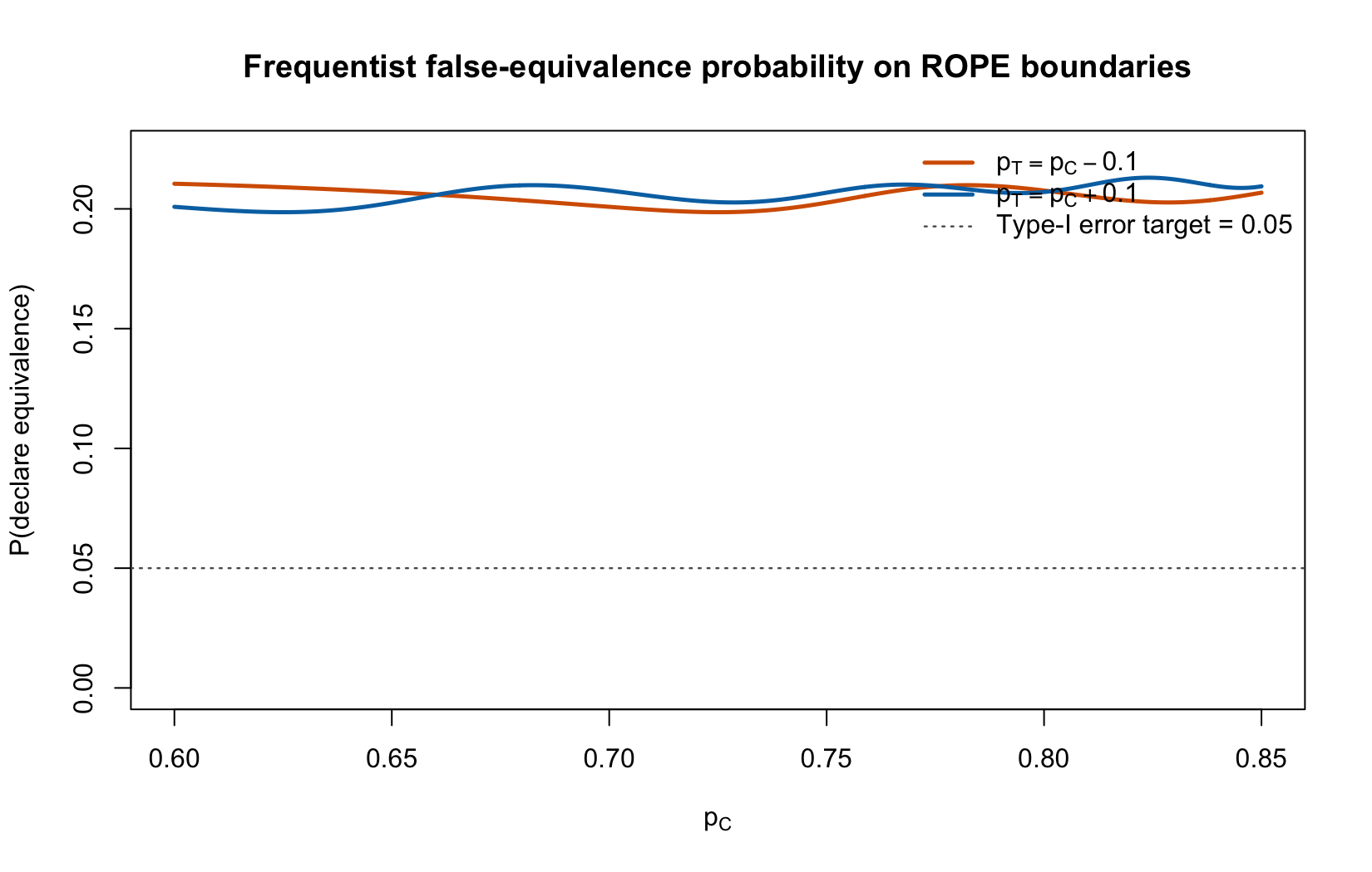
Figure 3: Visualization of the frequentist false-equivalence probability (a type-I-error) on the ROPE boundaries for the two-arm one-stage ROPE design for a binary endpoint.

Interpretation of the boundary-error diagnostic

Figure 3 evaluates the Bayesian-predictive design at

$$n_C=n_T=218, \qquad \gamma_{\mathrm{eq}}=0.80,$$

under a frequentist conditional-error perspective. The figure displays the probability of declaring equivalence when the true treatment-control risk difference lies exactly on either ROPE boundary:

$$p_T=p_C-0.10,$$

or

$$p_T=p_C+0.10,$$

for control-arm response probabilities in the clinically motivated interval

$$p_C\in[0.60,0.85].$$

At every point on these curves, the true absolute risk difference equals the ROPE half-width:

$$|p_T-p_C|=0.10.$$

Therefore, a declaration of equivalence at any of these parameter values is a false-equivalence decision under the frequentist null hypothesis.

The diagnostic shows that the probability of declaring equivalence can be much larger than 0.05 on the ROPE boundaries. For the present Bayesian-predictive design, the maximum boundary-grid probability is approximately

$$0.213.$$

More specifically, the largest value on the lower boundary is approximately

$$0.210,$$

at

$$(p_C,p_T)=(0.60,0.50),$$

whereas the largest value on the upper boundary is approximately

$$0.213,$$

at approximately

$$(p_C,p_T)=(0.824,0.924).$$

Thus, under some fixed parameter configurations that lie exactly on the practical-equivalence boundary, about 21% of repeated trials would declare equivalence using the Bayesian-predictive design.

This does not contradict the Bayesian predictive false-equivalence probability of 0.0434 reported for the same design. The two quantities answer different questions:

• The Bayesian predictive false-equivalence probability averages the conditional probability of declaring equivalence over the non-equivalence design distribution $G_0$.

• The boundary diagnostic evaluates the conditional probability of declaring equivalence at individual fixed parameter configurations and reports a maximum over the selected boundary grid.

A prior-weighted average can be small even when the conditional error probability is appreciably larger at particular parameter values. In this example, the non-equivalence design distribution $G_0$ does not assign all of its probability mass to the worst-case boundary configurations. As a result, averaging over $G_0$ yields a predictive false-equivalence probability below 0.05, whereas the maximum fixed-parameter boundary probability is about 0.21.

The figure therefore makes the calibration trade-off explicit. The $218+218$ Bayesian-predictive design is efficient when the design objective is good average decision performance under the clinically specified planning distributions. It is not designed to provide a conventional frequentist upper bound of 0.05 on the conditional false-equivalence probability at every ROPE-boundary value.

If pointwise frequentist boundary protection is required, the more stringent frequentist calibration described above should be used. In the present example, that approach increases the required sample size to $401+401=802$ participants and uses the stricter equivalence threshold $\gamma_{\mathrm{eq}}=0.975$.

Take-away

The two designs answer different questions:

1. Bayesian predictive calibration at $\gamma_{\mathrm{eq}}=0.80$ seeks a practical sample size while controlling the prior-weighted false-equivalence probability under a clinically specified non-equivalence design distribution.
2. Frequentist calibration at $\gamma_{\mathrm{eq}}=0.975$ seeks pointwise power at a fixed equivalence scenario and low maximum false-equivalence probability over a grid on the ROPE boundaries.

Neither calibration is universally preferable. The appropriate choice depends on whether the trial objective is framed as a predictive development decision under explicit clinical scenarios or as a design requiring pointwise frequentist error protection. The selected calibration criterion, design priors, ROPE, posterior thresholds, and all reported operating characteristics should be prespecified.

Hercogová, J., K. A. Papp, V. Chyrok, M. Ullmann, P. Vlachos, and C. J. Edwards. 2020. “AURIEL-PsO: A Randomized, Double-Blind Phase III Equivalence Trial to Demonstrate the Clinical Similarity of the Proposed Biosimilar MSB11022 to Reference Adalimumab in Patients with Moderate-to-Severe Chronic Plaque-Type Psoriasis.” Br. J. Dermatol. 182 (2): 316–26. https://doi.org/10.1111/bjd.18220.

Luterman, Maynard, Guy Tellier, Benjamin Lasko, and Bruno Leroy. 2003. “Efficacy and Tolerability of Telithromycin for 5 or 10 Days Vs Amoxicillin/Clavulanic Acid for 10 Days in Acute Maxillary Sinusitis.” Ear. Nose. Throat J. 82 (8): 576–80, 82–84, 586 passim.