Power and Sample Size Calculations for ROPE-based Non-Inferiority and Superiority Tests in Two-arm Clinical Trials with binary Endpoints

Riko Kelter
Institute of Medical Statistics and Computational Biology
Faculty of Medicine
University of Cologne
Cologne, Germany

28 October 2026

library(bfbin2arm)

Overview

This vignette illustrates the one-stage two-arm directional ROPE design for binary endpoints using two genuine, published clinical trials. The first example, ORIGINAL, is a classical non-inferiority trial with a regulatory-style margin derived from historical placebo-controlled evidence. The second example, SINGLE, is a nested non-inferiority/superiority trial that makes the distinction between non-inferiority power and superiority power explicit: the trial was powered for non-inferiority, and superiority was assessed only as a secondary, hierarchically nested claim.

Both designs use the risk difference $p_T - p_C$ as the effect measure. Non-inferiority is declared when the posterior probability of $p_T - p_C > -\delta_{\mathrm{ni}}$ reaches $\gamma_{\mathrm{ni}}$; superiority is declared, within the non-inferiority acceptance region, when the posterior probability of $p_T - p_C > \delta_{\mathrm{sup}}$ reaches $\gamma_{\mathrm{sup}}$.

Non-inferiority example: ORIGINAL stroke trial

ORIGINAL compared a modified alteplase regimen against standard alteplase for acute ischemic stroke, compare Meng et al. (2024b) and Meng et al. (2024a). The regulatory margin in the published protocol was specified on the risk-ratio scale, based on prior placebo-controlled alteplase evidence giving a relative risk of favorable outcome of 1.24 (95% CI 1.14 to 1.36). Preserving 50% of the conservative bound of that historical effect on the log-relative-risk scale gives the non-inferiority boundary

$$\mathrm{RR}_{\mathrm{ni}} = \frac{1}{\sqrt{1.14}} \approx 0.937.$$

Because this package’s two-arm directional engine is parameterized on the risk-difference scale, we translate this boundary locally at the trial’s planned control response rate $p_C = 0.63$:

$$\delta_{\mathrm{ni}} = p_C\,(1-\mathrm{RR}_{\mathrm{ni}}) = 0.63 \times (1 - 0.937) \approx 0.0397.$$

This linearization is only exact at $p_C = 0.63$; it is used here because the risk-ratio scale is not yet natively supported by the directional engine (a planned effect_scale = "risk_ratio" argument would allow an exact reproduction). The control-arm response rate itself was elicited from historical evidence in NOR-TEST and a Chinese alteplase cohort study, giving the planning value $p_C = 0.63$ used below, compare Meng et al. (2024b).

The design prior under non-inferiority assumes a small true improvement over the historical control rate, consistent with the trial’s planning assumptions; the design prior under harmful inferiority assumes a clinically important loss of efficacy at least as large as the margin.

design_prior_ni_original <- list(
  type = "baseline_difference",
  baseline = list(mean = 0.63, sd = 0.02, truncation = c(0, 1)),
  difference = list(mean = 0.028, sd = 0.01, truncation = c(-0.0397, 1))
)

design_prior_inf_original <- list(
  type = "baseline_difference",
  baseline = list(mean = 0.63, sd = 0.02, truncation = c(0, 1)),
  difference = list(mean = -0.08, sd = 0.02, truncation = c(-1, -0.0397))
)

First, we run a coarse sample size search using nstep = 25:

coarse <- design_twoarm_onestage_rope_ni(
     nmin = 200, nmax = 900, nstep = 25,
     delta_ni = 0.0397, gamma_ni = 0.95, gamma_inf = 0.95,
     analysis_prior_C = c(1, 1), analysis_prior_T = c(1, 1),
     design_prior_ni = design_prior_ni_original,
     design_prior_inf = design_prior_inf_original,
     target_ni_power = 0.80, target_false_ni = 0.05,
     calibration = "Bayesian",
     freq_ni_pC = 0.63,
     freq_ni_delta = 0,              
     target_freq_ni_power = 0.80,
     target_freq_false_ni = 0.05,  
     integration = "quantile",
     quad_nodes = 64L,
     parallel = TRUE, ncores = parallel::detectCores() - 1L,
     parallel_backend = "psock", progress = FALSE
)

coarse

One-stage two-arm ROPE non-inferiority design 
--------------------------------------------- 

Non-inferiority margin delta_ni: 0.0397 
Superiority margin delta_sup: 0 
Thresholds: gamma_ni = 0.95 , gamma_sup = 0.975 , gamma_inf = 0.95 

Selected design:
  nC = 650 , nT = 650 , N = 1300 

Target non-inferiority (or superiority) power: 0.8000 
Maximum predictive false non-inferiority probability: 0.0500 

Non-inferiority (or superiority) power, P(NI or sup | G_ni): 0.8028 
Superiority power, P(sup | G_sup): NA 
False non-inferiority probability, P(NI or sup | G_inf): 0.0039 
False superiority probability, P(sup | G_not_sup): NA 

Then, we refine the search by using nmin = 620, nmax = 670, nstep = 1:

original_ni <- design_twoarm_onestage_rope_ni(
  nmin = 620, nmax = 670, nstep = 1,
  delta_ni = 0.0397,
  gamma_ni = 0.95, gamma_inf = 0.95,
  analysis_prior_C = c(1, 1), analysis_prior_T = c(1, 1),
  design_prior_ni = design_prior_ni_original,
  design_prior_inf = design_prior_inf_original,
  target_ni_power = 0.80, target_false_ni = 0.05,

  calibration = "Bayesian",

  freq_ni_pC = 0.63,
  freq_ni_delta = 0,              
  target_freq_ni_power = 0.80,
  target_freq_false_ni = 0.05,    

  integration = "quantile", quad_nodes = 64L,
  parallel = TRUE, ncores = parallel::detectCores() - 1L,
  parallel_backend = "psock", progress = FALSE
)

We inspect the selected design.

original_ni
#> One-stage two-arm ROPE non-inferiority design 
#> --------------------------------------------- 
#> 
#> Non-inferiority margin delta_ni: 0.0397 
#> Superiority margin delta_sup: 0 
#> Thresholds: gamma_ni = 0.95 , gamma_sup = 0.975 , gamma_inf = 0.95 
#> 
#> Selected design:
#>   nC = 645 , nT = 645 , N = 1290 
#> 
#> Target non-inferiority (or superiority) power: 0.8000 
#> Maximum predictive false non-inferiority probability: 0.0500 
#> 
#> Non-inferiority (or superiority) power, P(NI or sup | G_ni): 0.8003 
#> Superiority power, P(sup | G_sup): NA 
#> False non-inferiority probability, P(NI or sup | G_inf): 0.0040 
#> False superiority probability, P(sup | G_not_sup): NA 
#> 
#> Pointwise frequentist non-inferiority power: 0.4367

The selected per-arm sample size, the non-inferiority power under the non-inferiority design prior, and the false non-inferiority probability under the harmful design prior can be inspected directly.

original_ni$nstar
#> [1] 645
original_ni$selected_fit$ni_power
#> [1] 0.8003392
original_ni$selected_fit$false_ni
#> [1] 0.003957997

Operating characteristics across the searched sample-size range can be plotted.

plot(original_ni)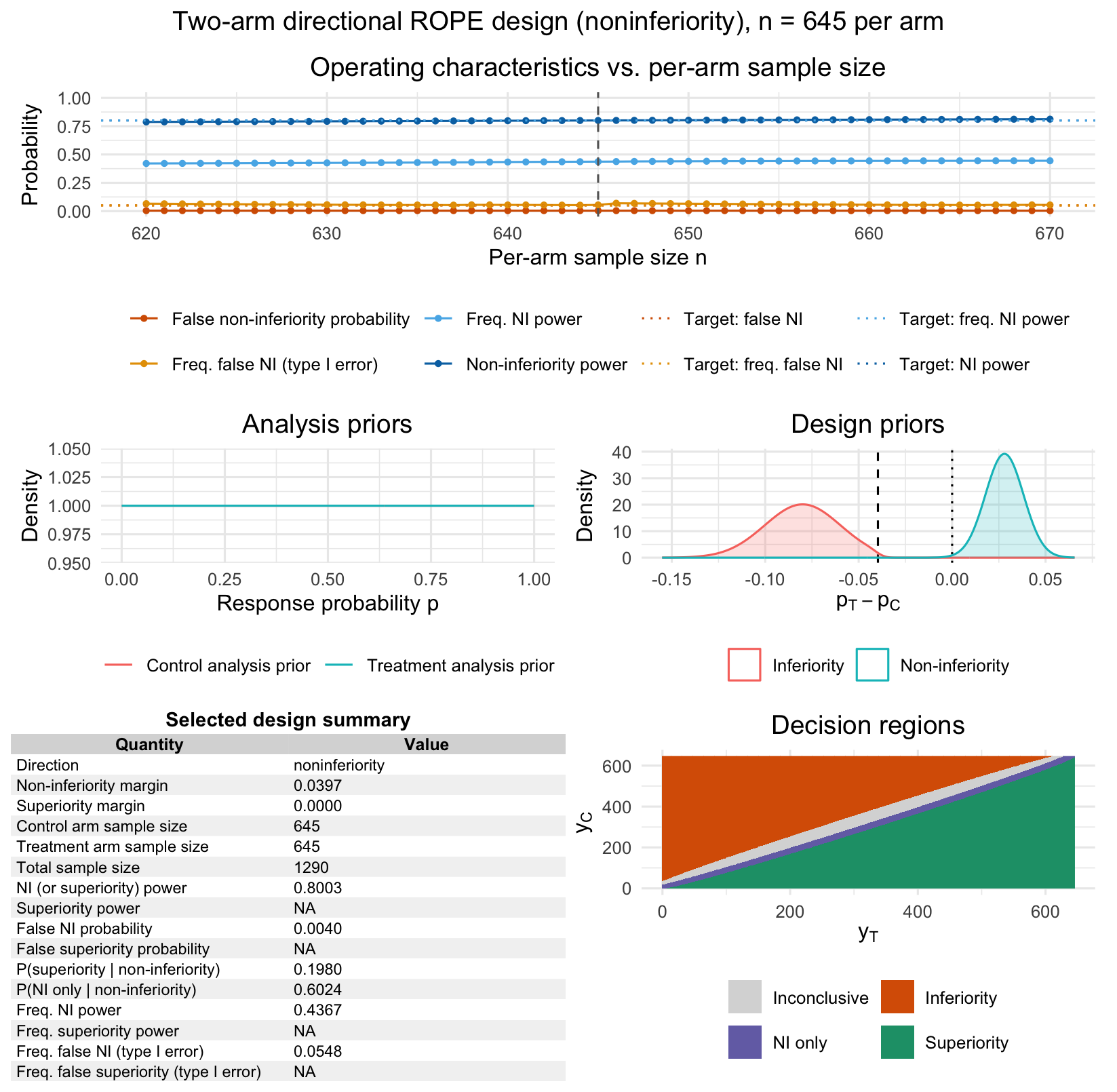

Figure 1: Output of the plot function for the non-inferiority single-arm one-stage ROPE design. The top left panel shows Bayesian and frequentist operating characteristics including type-I-error and power for varying sample sizes. The top right panel provides information about the calibrated design found by the calibration algorithm. The lower left and middle panels visualize the analysis and design priors under the inferiority and non-inferiority hypothesis. The bottom right panel displays the decision regions depending on the number of responses in the treatment and control arm.

Why superiority operating characteristics are not reported here

The summary above reports NA for the superiority power and the false superiority probability. This is expected, not an error, and reflects a deliberate feature of the directional calibration engine rather than a missing computation.

design_twoarm_onestage_rope_ni() calls the underlying directional engine with direction = "noninferiority". Under this direction, only two design priors are required and used: design_prior_ni, describing the predictive scenario under which non-inferiority is expected to hold, and design_prior_inf, describing a clinically important harmful scenario against which the false non-inferiority probability is evaluated. Neither design_prior_sup nor design_prior_not_sup was supplied in the call above.

The superiority power, $P(\text{superiority}\mid G_{\mathrm{sup}})$, requires integrating the posterior superiority decision rule against a design prior $G_{\mathrm{sup}}$ representing a true-superiority scenario. Because no such design prior was supplied, there is no distribution to integrate against, and the quantity is correctly reported as NA rather than silently defaulting to zero or some other placeholder value. The false superiority probability, $P(\text{superiority}\mid G_{\mathrm{not\_sup}})$, is NA for the same reason: it requires design_prior_not_sup, which was also not supplied.

This mirrors how ORIGINAL was actually designed and analyzed: it is a pure non-inferiority trial with no pre-specified superiority hypothesis, so a superiority operating characteristic would not be a meaningful quantity to report for this design. The threshold gamma_sup = 0.975 still appears in the printed summary, but only because it is used internally by the four-way decision matrix to classify each possible outcome $(y_C, y_T)$ into superiority, noninferiority_only, inferiority, or inconclusive. Since no design prior exists over which to average that classification for the superiority category specifically, the resulting power quantity has nothing to be averaged against, and remains undefined for this design.

The nested SINGLE example below in this vignette illustrates the contrasting case, where a superiority-relevant design prior is available and the distinction between non-inferiority power and superiority power becomes directly interpretable.

Nested non-inferiority/superiority example: SINGLE trial

SINGLE compared dolutegravir/abacavir/lamivudine against a ritonavir-boosted-atazanavir-based regimen in treatment-naive HIV-1 patients, compare Walmsley et al. (2013). The trial was designed with 90% power for a non-inferiority margin of $\delta_{\mathrm{ni}} = 0.10$ on the risk-difference scale, under the planning assumption of equal 75% response rates at week 48 in both arms. Because the design prior for non-inferiority assumed no true difference between arms, the trial’s superiority-related operating characteristic under that same scenario is far lower than its non-inferiority power: under exact equality, the probability of crossing the superiority threshold reduces to the nominal one-sided posterior threshold’s complement rather than to anything resembling 90%. The observed week-48 results, 88% for dolutegravir/abacavir/lamivudine versus 81% for the comparator, nevertheless crossed both the non-inferiority and superiority thresholds, which is why the trial was able to report superiority as a secondary finding.

We reproduce the nested design using the non-inferiority design prior only, and treat the probability of a superiority conclusion under that same design prior purely as a derived, secondary quantity. This mirrors how the trial was actually planned and reported: the primary calibration target is non-inferiority power, and the chance of a superiority conclusion under the planning scenario is read off, not separately targeted.

design_prior_ni_single <- list(
  type = "baseline_difference",
  baseline = list(mean = 0.75, sd = 0.02, truncation = c(0, 1)),
  difference = list(mean = 0, sd = 1e-6, truncation = c(-0.10, 1))
)

design_prior_inf_single <- list(
  type = "baseline_difference",
  baseline = list(mean = 0.75, sd = 0.02, truncation = c(0, 1)),
  difference = list(mean = -0.15, sd = 0.02, truncation = c(-1, -0.10))
)

The trial’s own sample-size calculation assumed no true difference between arms as the planning scenario for non-inferiority power — this is a very common convention in non-inferiority trial design, where the “worst realistic case” for powering the NI claim is taken to be exact equality, since that’s the scenario under which crossing the NI margin is hardest to guarantee with high probability (there’s no true benefit to lean on).

Setting difference sd = 1e-6 above creates an essentially degenerate point-mass prior at difference mean = 0, which is the direct translation of “assume equal response rates” into a design prior. It’s not meant to represent genuine uncertainty about the treatment effect — it’s meant to pin the calibration exactly at the specific scenario the original trial’s own power calculation used, so that the reproduction’s ni_power target (0.90) can be validated against the real, published sample size.

single_nested_coarse <- design_twoarm_onestage_rope_nisup(
  nmin = 200,
  nmax = 450,
  nstep = 5,

  delta_ni = 0.10,
  delta_sup = 0,

  gamma_ni = 0.95,
  gamma_sup = 0.95,
  gamma_inf = 0.95,

  analysis_prior_C = c(1, 1),
  analysis_prior_T = c(1, 1),

  design_prior_ni = design_prior_ni_single,
  design_prior_inf = design_prior_inf_single,

  target_ni_power = 0.90,
  target_false_ni = 0.05,

  calibration = "Bayesian",
  
  freq_ni_pC = 0.75,
  freq_ni_delta = 0,              
  target_freq_ni_power = 0.80,
  target_freq_false_ni = 0.05, 
  
  integration = "quantile",
  quad_nodes = 64L,
  parallel = TRUE,
  ncores = parallel::detectCores() - 1L,
  parallel_backend = "psock",

  progress = FALSE
)

We inspect the coarse fit:

single_nested_coarse$nstar
#> [1] 320

Thus, at $n=320$ per arm the target constraints were reached. Next, we refine the calibration, by setting nmin = 300 and nmax = 325 and nstep = 1:

single_nested <- design_twoarm_onestage_rope_nisup(
  nmin = 300,
  nmax = 325,
  nstep = 1,

  delta_ni = 0.10,
  delta_sup = 0,

  gamma_ni = 0.95,
  gamma_sup = 0.95,
  gamma_inf = 0.95,

  analysis_prior_C = c(1, 1),
  analysis_prior_T = c(1, 1),

  design_prior_ni = design_prior_ni_single,
  design_prior_inf = design_prior_inf_single,

  target_ni_power = 0.90,
  target_false_ni = 0.05,

  calibration = "Bayesian",
  
  freq_ni_pC = 0.75,
  freq_ni_delta = 0,              
  target_freq_ni_power = 0.80,
  target_freq_false_ni = 0.05, 
  
  integration = "quantile",
  quad_nodes = 64L,
  parallel = TRUE,
  ncores = parallel::detectCores() - 1L,
  parallel_backend = "psock",

  progress = FALSE
)

We inspect the fit:

single_nested
#> One-stage two-arm nested ROPE non-inferiority/superiority design 
#> ---------------------------------------------------------------- 
#> 
#> Non-inferiority margin delta_ni: 0.1 
#> Superiority margin delta_sup: 0 
#> Thresholds: gamma_ni = 0.95 , gamma_sup = 0.95 , gamma_inf = 0.95 
#> 
#> Selected design:
#>   nC = 318 , nT = 318 , N = 636 
#> 
#> Target non-inferiority (or superiority) power: 0.9000 
#> Maximum predictive false non-inferiority probability: 0.0500 
#> 
#> Non-inferiority (or superiority) power, P(NI or sup | G_ni): 0.9005 
#> Superiority power, P(sup | G_sup): NA 
#> False non-inferiority probability, P(NI or sup | G_inf): 0.0038 
#> False superiority probability, P(sup | G_not_sup): NA 
#> 
#> Pointwise frequentist non-inferiority power: 0.9000

Now, given the finer calibration search, $n=318$ patients is the first sample size at which the target constraints are met.

As with the ORIGINAL example above, sup_power and false_sup are reported as NA here. This design was calibrated with design_prior_sup and design_prior_not_sup left unspecified, since only a true-superiority scenario and a true-non-superiority scenario would allow those two quantities to be computed, and neither is part of how SINGLE was actually planned. The quantity of interest for demonstrating the non-inferiority power versus superiority power distinction is instead the probability of a superiority conclusion evaluated under the non-inferiority design prior, $P(\text{superiority}\mid G_{\mathrm{ni}})$, which is available directly from the nested decision breakdown below.

single_nested$nstar
#> [1] 318
single_nested$selected_fit$ni_power
#> [1] 0.900461
single_nested$selected_fit$p_sup_g_ni
#> [1] 0.04973937

The non-inferiority power at the selected sample size matches the trial’s planning target closely, while the probability of concluding superiority under that same, null design prior is far smaller, just 5%. This numerically demonstrates the distinction between non-inferiority power and superiority power: a design can be highly powered to conclude non-inferiority (90%) while having very little chance of concluding superiority (5%), if the design prior places its mass at or near equality.

The full four-way decision breakdown under the non-inferiority design prior shows how often each of the four possible conclusions (superiority, non-inferiority-only, inferiority, inconclusive) occurs under the trial’s own planning assumption.

c(
  superiority          = single_nested$selected_fit$p_sup_g_ni,
  noninferiority_only  = single_nested$selected_fit$p_ni_only_g_ni,
  inferiority           = single_nested$selected_fit$p_inf_g_ni,
  inconclusive          = single_nested$selected_fit$p_inc_g_ni
)
#>         superiority noninferiority_only         inferiority        inconclusive 
#>        4.973937e-02        8.507216e-01        2.475496e-06        9.953653e-02

plot(single_nested)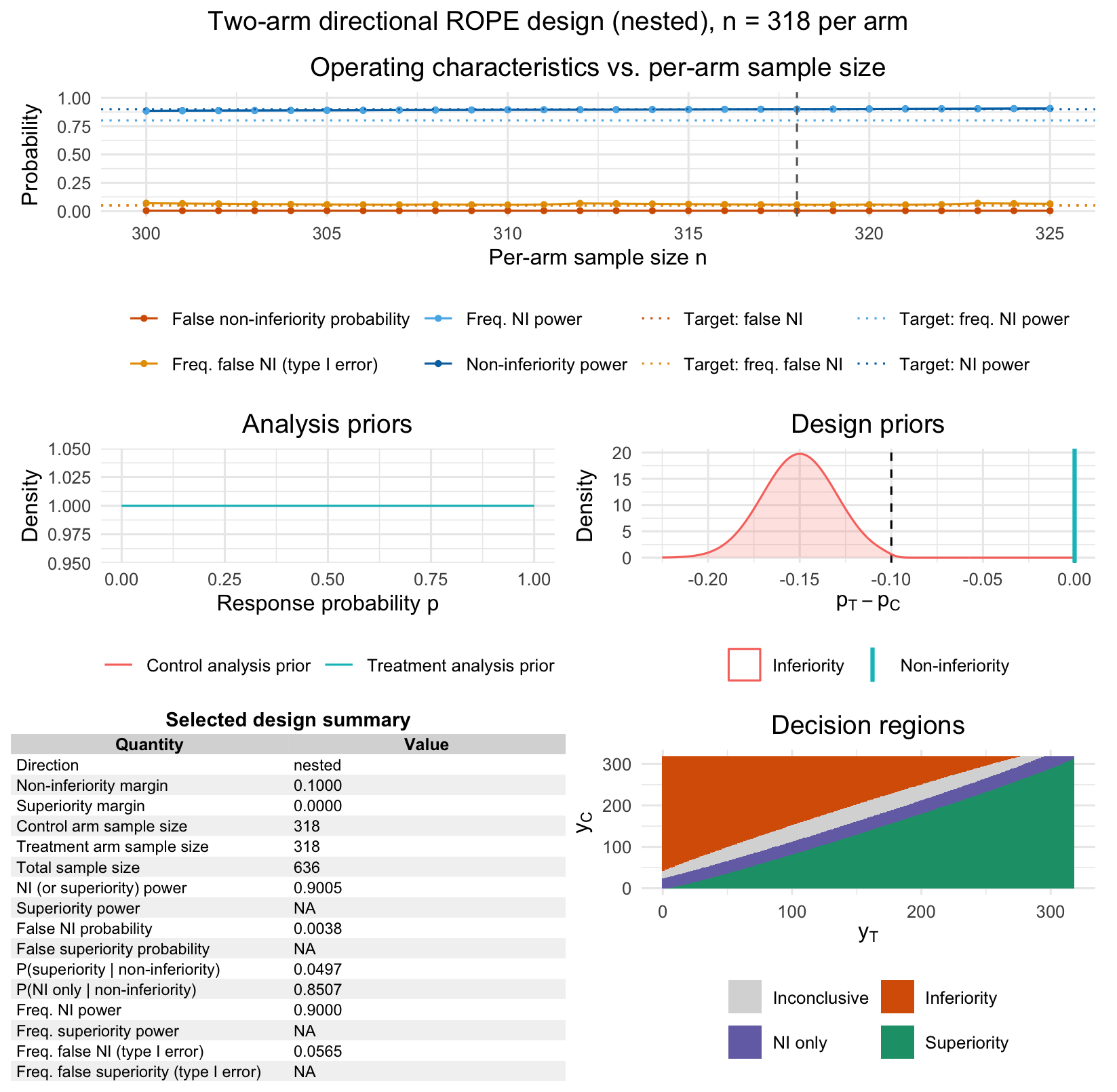

Figure 2: Output of the plot function for the nested non-inferiority-superiority single-arm one-stage ROPE design in the setting of the SINGLE trial. The top left panel shows Bayesian and frequentist operating characteristics including type-I-error and power for varying sample sizes. The top right panel provides information about the calibrated design found by the calibration algorithm. The lower left and middle panels visualize the analysis and design priors under the inferiority and non-inferiority hypothesis. The bottom right panel displays the decision regions depending on the number of responses in the treatment and control arm.

Checking the observed trial result against the calibrated design

The trial’s actual week-48 results can be evaluated directly against the calibrated design’s decision rule, using the observed responder counts at the trial’s actual per-arm sample sizes (419 on the comparator arm and 414 on the study arm).

nC_obs <- 419
nT_obs <- 414

yC_obs <- round(0.81 * nC_obs)
yT_obs <- round(0.88 * nT_obs)

decision_obs <- bfbin2arm:::.directional_decision_matrix_twoarm(
  nC_obs, nT_obs,
  delta_ni = 0.10, delta_sup = 0,
  gamma_ni = 0.975, gamma_sup = 0.975, gamma_inf = 0.975,
  analysis_prior_C = c(1, 1), analysis_prior_T = c(1, 1),
  integration = "quantile", quad_nodes = 64L
)

decision_obs$superiority[yC_obs + 1L, yT_obs + 1L]
#> [1] TRUE
decision_obs$noninferiority_only[yC_obs + 1L, yT_obs + 1L]
#> [1] FALSE

The observed data cross the superiority threshold, consistent with the trial’s own reported secondary superiority finding, even though the design was calibrated purely on non-inferiority power.

Comparing the two examples

Trial	Margin_scale	delta_ni	Control_rate_pC	n_per_arm_selected	ni_power	p_superiority_under_ni_prior
ORIGINAL (stroke)	Risk ratio, locally converted to RD	0.0397	0.63	645	0.8	NA
SINGLE (HIV)	Risk difference	0.1000	0.75	318	0.9	0.05

The table quantifies the central methodological point of this vignette. ORIGINAL is a pure non-inferiority design with no superiority-relevant design prior at all, so no probability of a superiority conclusion is reported. SINGLE, by contrast, is a nested design calibrated to reach 90% non-inferiority power, yet under the very same design prior used for that calibration, the probability of additionally concluding superiority is only 0.05. This large gap between a non-inferiority power of 0.900 and a superiority-conclusion probability of 0.05, evaluated under the identical design prior, is the numerical demonstration of why non-inferiority power and superiority power are distinct operating characteristics: a trial can be highly powered to establish non-inferiority while having very little chance of additionally establishing superiority, whenever the design prior places its mass at or near equality between arms. Consistent with this, the trial’s own week-48 results crossed the superiority threshold only because the observed treatment effect happened to fall well outside the design prior’s equality-centered scenario, not because the design was powered to detect it.

The table highlights the central methodological point of this vignette: ORIGINAL is a pure non-inferiority design with no superiority-relevant design prior at all, whereas SINGLE is a nested design in which the probability of a superiority conclusion is not separately targeted but instead follows, as a much smaller derived quantity, from the same design prior used to calibrate non-inferiority power. Even though the eventual decision in the SINGLE trial can additionally state superiority (next to the non-inferiority claim), the trial was originally not powered to detect superiority. If the goal would have been to detect superiority, a design calibration with a superiority and non-superiority design prior would have been appropriate instead.

References

Meng, Xia, Shuya Li, Hongguo Dai, et al. 2024a. “Tenecteplase Vs Alteplase for Patients With Acute Ischemic Stroke.” JAMA 332 (17): 1437–45. https://doi.org/10.1001/jama.2024.14721.

Meng, Xia, Shuya Li, Hongguo Dai, et al. 2024b. “Tenecteplase Vs Alteplase for Patients With Acute Ischemic Stroke: The ORIGINAL Randomized Clinical Trial.” JAMA 332 (17): 1437–45. https://doi.org/10.1001/jama.2024.14721.

Walmsley, Sharon L., Antonio Antela, Nathan Clumeck, et al. 2013. “Dolutegravir Plus Abacavir–Lamivudine for the Treatment of HIV-1 Infection.” New England Journal of Medicine 369 (19): 1807–18. https://doi.org/10.1056/NEJMoa1215541.